Deep Autocorrelation Modeling: The Secret Sauce of Time-Series Forecasting

TL;DR

Time-series forecasting is fundamentally different from image or text processing because of Autocorrelation—the statistical dependency of a variable on its own past. This survey by Wang et al. (2025) argues that the entire evolution of deep forecasting can be summarized by how we model this dependency in history (via architectures) and labels (via objectives). By bridging the gap between classical statistics and deep learning, the paper provides a roadmap for the next generation of "Autocorrelation-aware" foundation models.

Problem & Motivation: The "Autocorrelation Bias"

Most practitioners treat time-series forecasting as a standard regression problem, often defaulting to Mean Squared Error (MSE). However, the authors expose a critical theoretical flaw: MSE assumes that future time steps are conditionally independent.

In reality, if it rains at $t+1$, it is highly likely to rain at $t+2$. This is the Label Autocorrelation. When you use a "flat" loss like MSE, you suffer from Autocorrelation Bias, where the model ignores the structural shape of the future, leading to "jittery" or morphologically incorrect predictions even if point-wise errors are low.

Methodology: The Dual-Frontier of Modeling

The paper breaks down the technical landscape into two main pillars:

1. Modeling History (The "How to See")

Architectures have evolved to expand the Effective Receptive Field (ERF) to capture long-range dependencies:

• From RNNs to SSMs: Traditional LSTMs struggled with memory bottlenecks. Modern State Space Models (like Mamba) use structured dynamics to compress history losslessly.
• From Local CNNs to Large Kernels: Models like ModernTCN utilize massive kernels to "see" the entire history window at once, emulating Transformer capabilities with convolutional efficiency.
• Inverted Transformers (iTransformer): Unlike standard Transformers that treat time-steps as tokens, iTransformer treats the entire series as a token, capturing inter-variate correlations more effectively.

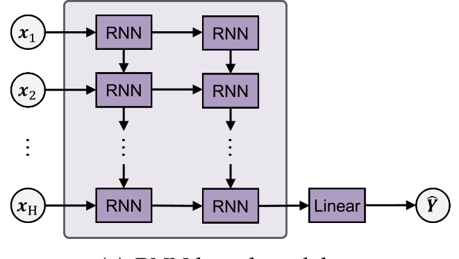Figure: Taxonomy of Non-Transformer architectures designed to capture historical dependency.

2. Modeling Labels (The "How to Learn")

This is the survey's most unique contribution—a systematic look at training objectives:

• Label Transformation: Methods like FreDF (Frequency domain) or Time-o1 (PCA) "whiten" the labels, turning a complex correlated sequence into independent components that are easier for MSE to handle.
• Shape Alignment: Utilizing SoftDTW, models learn to minimize morphological differences rather than just point-to-point distances.
• Distribution Balancing: Using Wasserstein Distance or GAN-based losses to ensure the distribution of the forecast matches the ground truth.

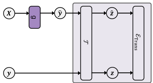Figure: The framework of Label Transformation and Covariance Modeling to mitigate autocorrelation bias.

Experiments & Results: The Rise of Foundation Models

The survey tracks how these concepts are converging into Large Time-Series Models (LTSMs).

• Success of Patching: Grouping time-points into tokens (PatchTST) has become the gold standard for Transformers, providing "local context" that raw points lack.
• Zero-shot Transfer: New foundation models (e.g., Chronos, TimesFM) trained on billions of data points are beginning to show that autocorrelation patterns found in "retail data" can, surprisingly, help in "energy forecasting" if the underlying temporal frequency is similar.

Table: Comparison of this work against prior surveys, highlighting the focus on Learning Objectives and Autocorrelation.

Critical Insight & Future Outlook

The paper concludes with a call to action: Modernize Canonical Statistics. Classical methods like Gaussian Processes and ARIMA were built on rigorous autocorrelation theory but don't scale. The next "breakthrough" will likely involve:

1. Lightweight Decorrelation: Using PCA-based layers to make simple linear models perform like deep nets.
2. Generative Refinement: Moving from Diffusion to Flow Matching (e.g., Sundial) for more stable and faster probabilistic forecasting.
3. Cross-domain Corpus: Creating 1-trillion+ point datasets to find the "universal constants" of autocorrelation.

Final Takeaway: If you are still training your Time-Series models with pure MSE, you are leaving performance on the table. It is time to align your loss functions with the geometric and statistical reality of your data.