TL;DR

Mixture-of-Experts (MoE) models offer the promise of high capacity with low compute costs, but their architectural design has long been a "black art" of heuristics. This paper changes that by establishing Holistic Scaling Laws. By reducing the design space from 16 dimensions to just a few manageable ratios, the authors provide a closed-form blueprint to determine the optimal depth, width, and expert configuration for any given compute budget.

Key Insight: As you scale up, the "optimal" configuration becomes more of a flexible "band" than a narrow peak, giving engineers the freedom to prioritize hardware efficiency without sacrificing model quality.

The Curse of Dimensionality in MoE

In traditional dense Transformers, scaling is relatively simple: you balance FLOPs (M) and parameters (N). In MoE, the triad of FLOPs (M), Active Parameters (Na), and Total Parameters (N) creates an entangled web.

Prior works typically took two paths:

1. The Brute Force Path: Adding MoE variables directly into scaling formulas, leading to an explosion of coefficients that are nearly impossible to fit accurately.
2. The Isolation Path: Fixing everything but the experts, which ignores the critical interaction between the attention layers and the expert blocks.

The authors argue that anchoring solely on FLOPs per token (M) is biased. MoE models can "inflate" their parameter counts to boost performance without increasing FLOPs, making fair comparisons impossible without a multi-dimensional constraint.

Methodology: The Art of Dimensionality Reduction

To solve the O(n^16) complexity problem, the authors systematically collapsed the search space:

1. Classical Alignment: They first re-fit the (C, M, D) scaling laws to map compute budget directly to model size (M) and data (D).
2. Algebraic Constraints: By fixing hardware-constrained values (like attention head dimensions) and using architectural equations, they reduced the problem to 4 degrees of freedom: M, Na, N, and the hidden dimension d.
3. The Proxy Shortcut: They discovered a rank-preserving property: the relative performance of different (M, Na, N) triplets stays the same regardless of the hidden dimension choice. This allowed them to use a "median proxy" for d to find the optimal triplet first, then fine-tune d later.

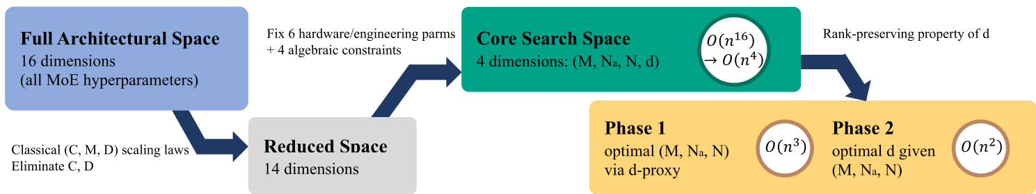Figure 1: The pipeline for collapsing the 16D architectural space into a manageable two-phase search.

Experimental Results: Finding the "Optimal Basin"

The team trained over 670 models. By visualizing the loss in the (M/Na, N/Na) plane, they identified a clear "low-loss basin."

• Optimal M/Na: Represents compute density. The study found that as the compute budget grows, the optimal M/Na (how much compute we spend per active parameter) actually decreases slightly.
• Optimal N/Na: Represents parameter expansion. Interestingly, the optimal N/Na ratio (total parameters vs. active parameters) proved remarkably stable between 18 and 25 across all scales.

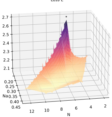Figure 2: The loss landscape in the transformed (M/Na, N/Na) coordinate system, showing the optimal design region.

Engineering Insight: The Widening Near-Optimal Band

Perhaps the most valuable contribution for practitioners is the analysis of the near-optimal band.

In small-scale models, architectural choices like the hidden dimension (d) are critical; being slightly off the optimum results in significant loss spikes. However, as the compute budget moves toward 3 × 10^20 FLOPs and beyond, this band widens. This means that for massive models, engineers can shift d to a power of 2 (e.g., 4096 or 8192) to maximize GPU kernel efficiency without worrying about a performance penalty.

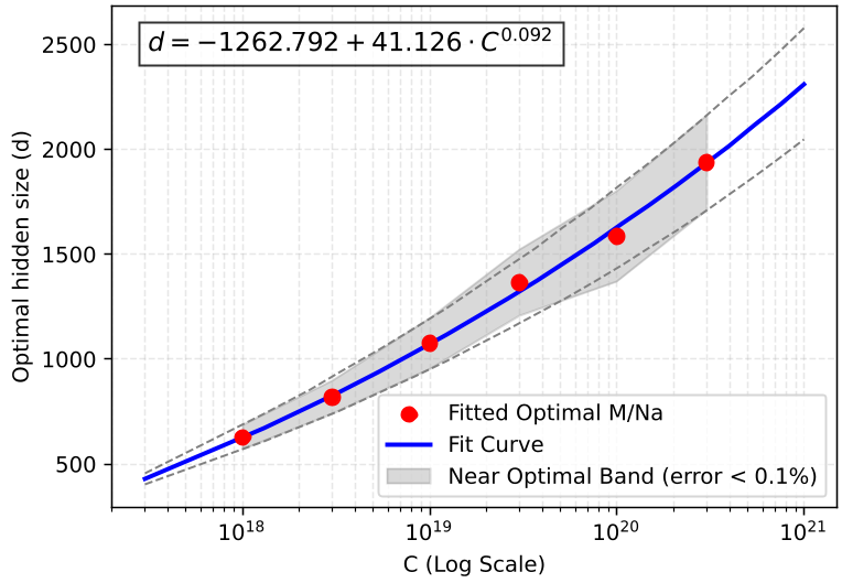Figure 3: The widening of the near-optimal band as compute scale increases, providing quantitative proof for engineering flexibility.

Critical Analysis & Conclusion

This work transitions MoE research from qualitative observation to quantitative engineering. However, there are inherent limitations:

• Fixed Sparsity: The experiments utilized a fixed expert configuration (8 active out of 288). While the framework is reusable, the specific coefficients might shift for different routing strategies (e.g., DeepSeek's shared experts).
• Pre-training vs. Downstream: The laws are based on cross-entropy loss. As recent literature suggests, loss does not always correlate perfectly with reasoning or specialized task performance.

Takeaway: This paper provides the first end-to-end pipeline to design MoE models from scratch based on a compute budget. It proves that the "correct" architecture is not a static point, but a scale-dependent target that becomes more forgiving as we push the frontiers of AI.