MoFI-FLR: Dissecting the "Simple" from the "Complex" in High-Dimensional Functional Data

TL;DR

In modern data science, we often face a dilemma: do we assume a simple, interpretable linear relationship, or do we go "full nonparametric" and risk overfitting? MoFI-FLR (Model Form Identification in Functional Linear Regression) solves this by using a clever two-stage framework. It doesn't just ask if a variable is important; it asks how it is important—identifying whether a functional predictor has a simple parametric effect or a complex, non-linear one.

Background: Beyond the Binary of Variable Selection

In high-dimensional functional data—like EEG signals or continuous environmental monitoring—the number of predictors $p$ often exceeds the sample size $n$. Existing methods are great at "Sparsity" (finding which predictors matter), but they treat all "active" predictors as black-box nonparametric functions.

The authors argue that this is a missed opportunity for Interpretability. For instance, in energy prediction, temperature might have a constant (simple) effect on base usage but a complex, time-varying effect during peak hours. MoFI-FLR is the first unified framework to bridge this gap in functional linear models.

Methodology: The Elegance of RKHS Decomposition

The core innovation lies in the Orthogonal Decomposition of the Reproducing Kernel Hilbert Space (RKHS).

1. The Two-Step Workflow

• Step 1: The Screen. Use a functional elastic-net penalty to filter out the "noise" variables (those with zero coefficients).
• Step 2: The Identification. For the remaining variables, split the coefficient function ${\beta }_j(t)$ into: ${\beta }_j(t)={\beta }_j^{(0)}(t)+{\beta }_j^{(1)}(t)$ Where ${\beta }_j^{(0)}$ is the simple component (e.g., constant, linear, or a few Gaussian bases) and ${\beta }_j^{(1)}$ is the complementary component (the "messy" nonparametric part).

2. Selective Penalization

The genius of the method is that the second stage applies regularization only to the complementary component ${\beta }_j^{(1)}$. If the data doesn't strongly support a complex relationship, the penalty shrinks ${\beta }_j^{(1)}$ to zero, leaving you with a perfectly interpretable, simple model form.

Theoretical Guarantees: Why It Works

The paper provides a non-asymptotic theory showing that the probability of correctly identifying the true model form (Null vs. Simple vs. Complex) converges to 1 as $n$ increases, even in ultra-high-dimensional regimes where $\log p=O(n^{1-2\varsigma })$.

One fascinating insight: The penalty required for form identification (Step 2) is actually smaller than the penalty for variable selection (Step 1). This makes intuitive sense—once you've cleared the "forest" of irrelevant variables, you can use a finer scalpel to dissect the remaining signals.

Experimental Proof: EEG and Brain-Behavior Latency

The authors put MoFI-FLR to the test using the Psychomotor Vigilance Task (PVT) EEG dataset.

• The Task: Predict reaction time from neural voltage trajectories across 42 channels.
• The Findings: The model identified 13 channels as "Simple" (well-captured by three Gaussian basis functions representing P1, P2, and P3 components) and others as "Complex."

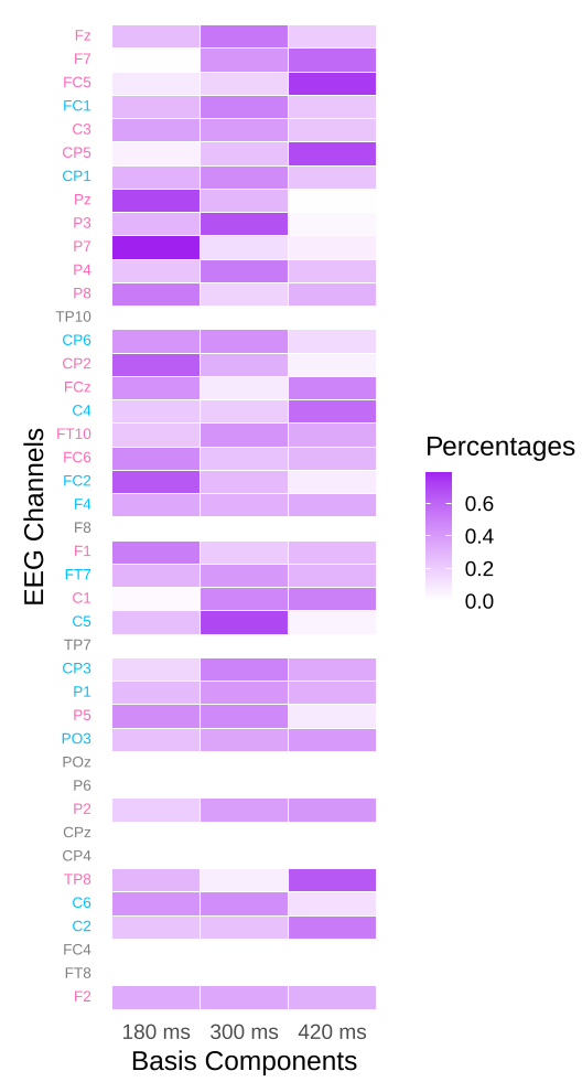In the figure above, note how channel FC1 is categorized as "Simple" because its effect is effectively captured by standard Gaussian bases, whereas C3 shows a "Complex" complementary component near the 600ms mark.

Critical Insight & Conclusion

MoFI-FLR isn't just a statistical tool; it’s a mindset shift for functional data analysis. By embedding scientific prior knowledge (like specific ERP windows in neuroscience) into the "Simple" subspace $H_{0j}$, we can test whether biological reality conforms to our theories or requires a more nuanced, nonparametric explanation.

Limitations: The model currently assumes functional predictors are fully observed. In many real-world scenarios, we only have sparse, noisy observations of the functions. Future extensions to "errors-in-variables" settings or discretely sampled data will be crucial for broader adoption in clinical settings.

Takeaway: If you are working with high-dimensional time-series or functional data, don't just ask which sensors are active. Use MoFI-FLR to discover which relationships are elegantly simple and which are essentially complex.