
Reinstating Layer Dropout for Compute-Efficient and Depth-Elastic LLM Pretraining
9.11:2
This paper revisits layer dropout for decoder-only LLM pretraining and finds that jointly tuned dropout scaling, whole-layer per-sequence granularity, an increasing-depth distribution, and a decreasing time schedule can preserve or improve validation loss while reducing training FLOPs. At large scale, the recommended recipe yields up to 25 percent training FLOPs savings and up to 1.55 times self-speculative inference speedup while inducing robustness to early exit and layer skipping.
TL;DR
This paper studies layer dropout in large-scale decoder-only LLM pretraining and argues that its historical rejection was premature because dropout was rarely configured jointly with optimizer transfer rules, granularity, depth distribution, and temporal schedule. Across more than 2400 training experiments, spanning 271M to 8.2B parameters and datasets up to 160B tokens, the authors find that whole-layer, per-sequence dropout with training scale inverse to layer density and a high initial dropout rate is the key stabilizing choice. The best recommended recipe is increasing dropout across depth and decreasing dropout across training steps, giving lower or similar validation loss while saving up to 25 percent of training FLOPs and enabling up to 1.55 times self-speculative decoding speedup (abstract and Table 5).
Background Positioning
This is not a new architecture or a new loss function. Its position in the literature is closer to a large-scale empirical systems paper that turns a known trick, stochastic depth or layer dropout, into a practical pretraining recipe. Earlier work such as LayerDrop and LayerSkip demonstrated benefits for elastic inference, but the modern LLM setting differs in three ways: single-epoch or near-single-epoch data, much larger token budgets, and stronger expectations about stable hyperparameter transfer across model scales. The paper’s main contribution is a controlled, cross-scale study that identifies which dropout variants actually survive the modern regime and which fail because of confounded implementation choices.
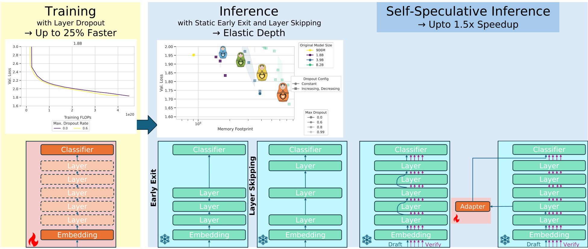
Figure 1 summarizes the thesis: stochastic depth in training is not merely a regularizer, but a mechanism for building a model whose effective depth can be varied at inference time with graceful degradation.
Problem and Motivation
The central confusion in this area is that dropout has several meanings, and the evidence against dropout is often evidence against activation dropout or poorly configured dropout. As LLMs scale to billions of parameters and trillions of tokens, models usually see each token once, which weakens the classical case for explicit regularization. Recent work cited in the introduction further claims that activation dropout can degrade performance in large-data regimes. This observation has been overgeneralized to dropout broadly, including structured layer dropout. The paper’s motivation is to separate these cases: activation dropout may be unnecessary, but layer dropout has a distinct property, because skipping an entire transformer block reduces active non-embedding FLOPs almost linearly when training is compute-bound.
The practical failure mode is also subtle. A model trained with 20 percent layer dropout is not the same as a model trained with a different optimizer configuration; its effective depth during early training is lower, its gradient distribution is altered, and its initialization scale may be mismatched to its effective depth. Prior papers that reported degradation may have changed the dropout rate without re-tuning learning rate, weight decay, batch size, or the dropout scaling convention. The introduction explicitly identifies this as an unresolved joint problem: should layer dropout be used in modern LLM training, and if so, how should it be configured to preserve accuracy while delivering training and deployment benefits?
The authors’ intuition is partly theoretical and partly empirical. The theoretical anchor is the CompleteP-style idea that residual updates should scale with effective depth for stable transfer across model depths. The empirical anchor is that dropout schedules and optimizer settings interact strongly enough to explain many earlier negative results. This makes the work best understood as an analysis-and-practice paper rather than a purely theoretical contribution.
Core Analysis: A Unified Empirical Account of Layer Dropout
Measurement: Stochastic Block Skipping as Effective-Depth Control
For a residual layer at training step , the paper writes the standard update as:
where is the activation tensor at that depth, is the layer function, and the residual connection passes the previous representation forward. With layer dropout, the update becomes stochastic:
Here is a binary mask for sequence , is the dropout probability, is layer density, and is a scaling factor. When the mask is zero for a sequence, the block computation is skipped for that sequence; when it is one, the output is added to the residual stream. The efficiency claim depends on not computing for masked sequences rather than merely multiplying by zero after the fact. The average dropout over depth at a given step can be summarized as the active FLOPs savings proxy:
In this expression, is the number of training steps, is depth, and is the dropout rate applied at layer and step . The quantity is the time-averaged, depth-averaged dropout probability, which the paper uses to group configurations with the same total non-embedding FLOPs savings. If , then roughly 5 percent of the layer-computation budget is removed under the paper’s compute-bound assumption. If all , the formula collapses to the dense baseline; if all are constant over depth and time, the savings are just that constant rate. The importance of this metric is that it exposes confounds: two runs with the same maximum dropout can have very different total compute exposure, so comparisons must be grouped by or training FLOPs savings rather than by peak dropout alone.
Design Choices: Hyperparameter Transfer, Granularity, Distribution, and Schedule
The first design choice is scaling. The paper argues that the choice of is critical:
where is the probability that a layer is retained. The scaling ensures that, for a sequence that does execute the layer, the residual update is boosted to match the expected contribution of a dense stream as dropout changes effective depth. The paper contrasts this with other conventions: Hinton-style dropout uses and an inference correction; PyTorch and TensorFlow use for activation dropout; DINOv2 uses ; torchtune-style LayerSkip implementations may use both scales set to 1. For this work, the authors set and , so that inference is the dense expectation of the stochastic training operation. Section 5 and Figures 2 and 3 report that with this choice, optimal learning rate, batch size, and weight decay remain largely constant across small to medium dropout rates, while requires per-rate tuning and violates stable coordinate checks.
The second choice is granularity. The paper distinguishes sub-layer dropout, where attention and FFN blocks can be dropped independently, from layer dropout, where a whole transformer block is dropped. Table 1 shows that layer dropout gives lower validation loss than sub-layer dropout at both 271M and 503M parameters. For example, at 271M and dropout 0.1, sub-layer dropout gives validation loss 2.377 while whole-layer dropout gives 2.367, both relative to a dense validation loss of 2.294. The authors also distinguish per-batch masking from per-sequence masking; Figure 4 reports that per-sequence dropout lowers validation loss. This result is intuitive because per-sequence masking exposes the model to finer-grained combinations of active paths, but the paper also notes a systems tradeoff: per-batch masking can avoid loading skipped weights, while per-sequence masking only gives similar wall-clock savings when training is compute-bound.
The third choice is depth distribution. The paper compares uniform dropout across layers, increasing layer distribution (ILD), and alternating layer distribution (ALD). The recommended increasing form is:
This means the first layer is never dropped, and the last layer is dropped with probability . The average over depth is , so a fixed corresponds to a maximum rate twice the average. Uniform dropout is not the best empirical choice: Table 2 groups configurations with equal FLOPs savings and finds that non-uniform distributions usually outperform uniform ones. At 20 percent FLOPs savings for the 906M model, uniform gives validation loss 2.008, ALD gives 2.004, and ILD gives 1.998. The paper notes that ALD can be best at the smallest scale for skip robustness, but as models grow, ILD’s advantage over uniform widens, which is why ILD becomes the recommended distribution for base accuracy and early exit robustness.
The fourth choice is temporal schedule. The winning schedule decays dropout over training:
where is the selected depth-wise rate, such as ILD. This linear decay ends in a dense model at the final training step. For ILD combined with a decreasing schedule, the depth average is and the time average is , so the total average dropout is . Thus a maximum rate of 0.2 corresponds to about 5 percent total FLOPs savings, while a maximum rate of 0.8 corresponds to about 20 percent. This schedule choice matters more than one might expect: Table 3 shows that for the same FLOPs savings, decreasing schedules consistently outperform constant and increasing schedules, while increasing schedules can substantially worsen loss.
Attribution and Counterfactuals: Why the Recipe Works and Where It Fails
The mechanism can be understood as stochastic model growing or curriculum learning. The paper hypothesizes that high dropout at the beginning of training creates a smaller effective depth, which forces the model to explore weight space with more noise and fewer redundant paths, while the decay to zero lets the model settle into a dense final minimum. This explanation is qualitative, not proven: the evidence is the consistent loss curve behavior across scales. A useful counterfactual is increasing time schedule. It preserves the same total compute savings in many grouped rows but yields worse validation loss. At 906M and 5 percent savings, ILD with increasing schedule gives validation loss 1.979, whereas ILD with decreasing schedule gives 1.951. At 10 percent savings, increasing schedule gives 2.014 while decreasing schedule gives 1.955. In other words, it is not merely the total exposure to sparsity that matters; the ordering of exposure during optimization determines whether the model benefits or degrades.
The distribution tradeoff is also mechanistically meaningful. ILD protects early layers and progressively skips deeper ones, which aligns well with base validation loss and early exit. ALD skips alternate layers, which gives better robustness for non-contiguous intermediate layer skipping but worse early exit behavior. The paper makes this tradeoff explicit in Section 8 and recommends choosing based on deployment mode: ILD plus decreasing schedule is the best general recipe, while ALD may be preferable when the main target is intermediate layer skipping. This is an unusually clean finding for practical model deployment: the same structural sparsity mechanism induces different inference elasticities, and the optimal training configuration depends on the inference-time budgeting method.
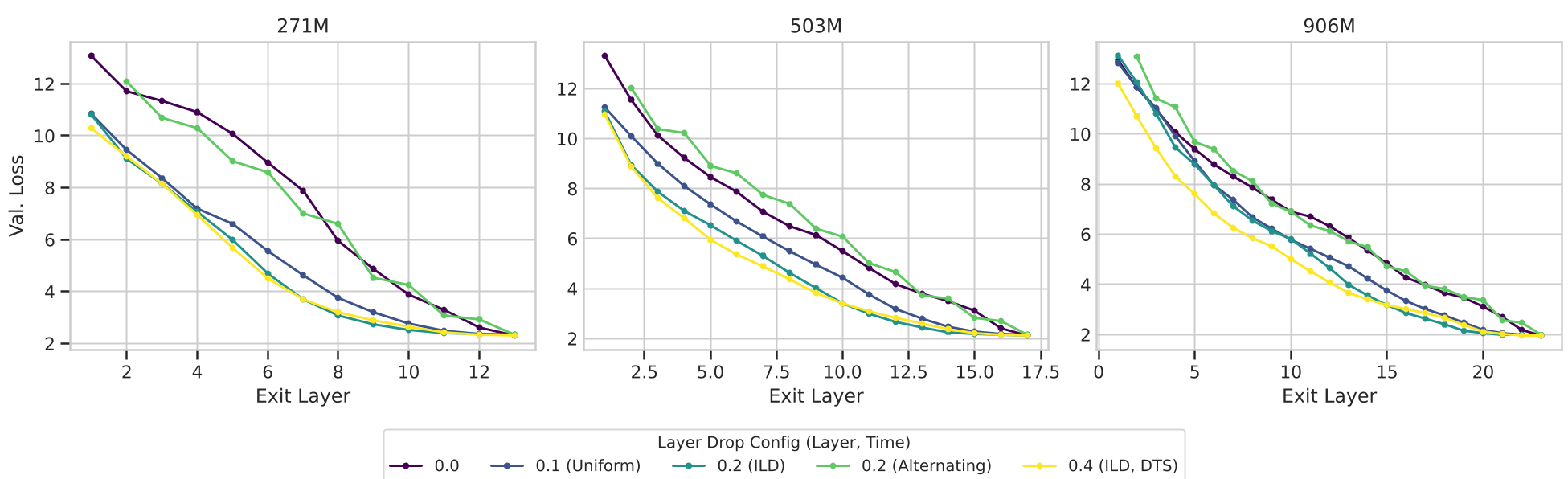
Figure 5 supports the early-exit claim: models trained with dropout degrade far more gracefully when exiting before the final layer, and a decreasing schedule does not erase the robustness learned during earlier dropout exposure.
Experiment and Evidence
The strongest quantitative evidence comes from controlled comparisons in Table 3, where configurations are grouped by equal training FLOPs savings and evaluated at 20 tokens per parameter. The following excerpt for the 906M model captures the central schedule result:
Table 3 reports validation loss and change versus the dense baseline at 20 TPP for the 906M model under configurations that share the same active non-embedding FLOPs reduction:
| FLOPs savings | Layer distribution | Time schedule | Max dropout | Validation loss | Change vs dense |
|---|---|---|---|---|---|
| 0 percent | Dense | None | 0 | 1.953 | 0.00 percent |
| 5 percent | Increasing | Constant | 0.1 | 1.961 | plus 0.42 percent |
| 5 percent | Increasing | Increasing | 0.2 | 1.979 | plus 1.34 percent |
| 5 percent | Increasing | Decreasing | 0.2 | 1.951 | minus 0.06 percent |
| 10 percent | Increasing | Constant | 0.2 | 1.972 | plus 1.01 percent |
| 10 percent | Increasing | Increasing | 0.4 | 2.014 | plus 3.15 percent |
| 10 percent | Increasing | Decreasing | 0.4 | 1.955 | plus 0.10 percent |
| 20 percent | Increasing | Decreasing | 0.8 | 1.983 | plus 1.55 percent |
The pattern is striking. At 5 percent savings, the proposed ILD plus decreasing schedule slightly beats the dense baseline, validating loss 1.951 versus 1.953. At 10 percent savings, it is almost equal to dense, within 0.002 validation loss, while the increasing schedule is 0.061 above the best decreasing configuration at the same budget. At 20 percent savings, degradation remains visible, but the decreasing schedule is clearly better than the uniform and increasing alternatives in the grouped table. These numbers directly support the paper’s central claim: layer dropout is not inherently harmful if the schedule and distribution are chosen correctly.
The second major evidence block is the large-scale “hero runs” in Table 5. These tests push maximum dropout to aggressive values at larger model sizes while keeping TPP at 20. The table reports validation loss, layer-skipping robustness, early-exit loss, and speculative-decoding speedup:
Table 5 compares dense and dropout-trained larger models at 20 TPP, with increasing depth distribution and decreasing time schedule for dropout runs:
| Configuration | Max dropout | FLOPs savings | Validation loss | Skip alternate loss | Early exit at 0.75 depth | Speculative speedup |
|---|---|---|---|---|---|---|
| 1.8B dense | 0 | 0 percent | 1.849 | 4.260 | 3.943 | 1.10x |
| 1.8B ILD plus DTS | 0.6 | 15 percent | 1.836 | 2.282 | 2.329 | 1.34x |
| 3.9B dense | 0 | 0 percent | 1.732 | 6.446 | 3.834 | 1.02x |
| 3.9B ILD plus DTS | 0.8 | 20 percent | 1.745 | 2.129 | 2.143 | 1.54x |
| 8.2B ILD plus DTS | 0.99 | 25 percent | 1.663 | 1.991 | 1.777 | 1.55x |
For the 1.8B model, dropout training saves 15 percent of layer computation and actually lowers validation loss from 1.849 to 1.836. For the 3.9B model, validation loss rises slightly from 1.732 to 1.745, but the inference robustness improves dramatically: skipping alternate layers drops from loss 6.446 to 2.129, and early exit at 0.75 depth drops from 3.834 to 2.143. The 8.2B run is the most aggressive: maximum dropout 0.99, which means the final layer is skipped nearly always during early training, still yields validation loss 1.663 with 25 percent FLOPs savings and 1.55 times speculative speedup. These results are not merely efficiency claims; they show a quality-elasticity coupling that dense training fails to provide.
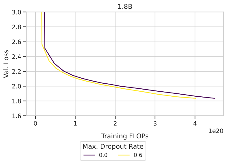
Figure 9 supports the same conclusion from the compute-loss perspective: under aggressive maximum dropout rates, training with layer dropout reaches lower validation loss for a given training FLOPs budget throughout most of the run.
The inference evidence connects to specific post-training mechanisms. Table 4 shows that at 504M and 20 TPP, a 0.4 ILD run obtains 1.43 times speculative decoding speedup with 97 percent acceptance rate and a draft-to-target time ratio of 0.42, compared with 1.03 times speedup and 90 percent acceptance for the dense baseline. This matches the broader claim in Section 8: average dropout during training predicts zero-shot robustness to depth reduction. The paper also evaluates early-exit adapters using Balcony-style frozen-backbone adapters; Figure 7 reports that dropout-pretrained backbones achieve better early-exit losses even after adapters are added post-training. That is a strong evidence line because it shows the benefit persists after further fine-tuning-like optimization on top of the pretrained weights.
The evidence quality assessment has to be nuanced. The controlled ablations mostly sit at 20 tokens per parameter, which is the compute-optimal budget in the paper’s setup, and the scaling analysis extends this into higher TPP regimes with Fig. 8 showing that ILD plus DTS degradation typically stays around 0.50 percent relative to baseline even at high TPP. The downstream results in Table A.3 are broadly competitive, with some tasks improving and others moving slightly, so the cleanest quantitative wins are validation loss, FLOPs savings, and elastic-depth metrics. The paper is also explicit that it does not compare against learned depth mechanisms such as Mixture-of-Depths, does not cover Mixture-of-Experts or non-transformer architectures, and does not yet derive scaling laws for the maximum dropout rate. Those are not hypothetical omissions; they are stated limitations, and they bound how strongly the paper can claim a universal pretraining recipe.
Deep Insights and Conclusion
The real contribution is not “dropout helps” but the identification of a specific failure taxonomy for prior dropout skepticism. The paper shows that layer dropout is sensitive to at least four interacting axes: scaling convention, tensor granularity, depth distribution, and temporal schedule. If the training scale is wrong, hyperparameter transfer breaks. If masking is per-batch rather than per-sequence, accuracy can suffer. If the depth distribution is uniform rather than increasing, the model wastes robustness in early layers or fails to protect early computation. If the time schedule increases rather than decreases, the same average sparsity can become harmful instead of beneficial. Table 3 is the clearest proof of this point: the same FLOPs savings category can range from beating dense by a tiny margin to losing more than three percent in relative validation loss, purely due to distribution and schedule.
The practical recommendation is unusually concrete. For modern LLM pretraining, use whole transformer-layer dropout sampled per sequence, with and , tune optimizer hyperparameters on a small model and transfer them using the paper’s µP and CompleteP-style rules, set the layer distribution to ILD, and schedule dropout to decay linearly to zero by the end of training. Then choose maximum dropout according to the desired savings and inference mode: 5 percent total savings already allows a small model to match dense loss, while aggressive regimes at multi-billion scale unlock large speculative-decoding and layer-skipping advantages. The tradeoff is that ALD may be better for non-contiguous intermediate skipping, while ILD is better for base loss and early exit. This means there is no single universally optimal dropout pattern; the correct choice depends on whether the deployment stack will cut depth from the tail, skip internal blocks, or train a draft subset for self-speculative decoding.
The limitations are meaningful and falsifiable. The authors themselves report that hyperparameter transfer degrades at very high dropout because learning rate and weight decay shrink away from the stable small-dropout region, and that their transfer analysis was mainly validated for constant schedules rather than the optimal decreasing schedule. They also have not quantified the scaling of inference benefits with TPP, nor compared their stochastic approach to learned routers or Mixture-of-Depths. In other words, the paper establishes a strong practical recipe but not a full scaling law for “how much dropout can a model absorb at size and token budget .”
The most interesting future direction is not merely “try dropout in another model,” but using the same principle as a generalized curriculum: the paper frames its recipe as stochastic model growing, where effective capacity increases through training. That view naturally extends to width, quantization bit-width, attention-head dropping, and possibly other structured capacity knobs. If the decreasing schedule works because early noise encourages exploration and late density stabilizes convergence, then one should expect similar effects wherever capacity, precision, or path diversity can be annealed. This is where the work becomes more than a dropout ablation: it proposes a training-time mechanism for manufacturing inference-time elasticity without adding architectural complexity, extra losses, or post-hoc pruning.