Scaling Laws 2.0: Optimizing the Token Allocation Strategy

TL;DR

The "Chinchilla" era taught us how much data and how many parameters we need. This paper teaches us how to spend those tokens. By introducing a Three-Term Law, the authors prove we can predict optimal batch sizes with 70% less compute, while finally reconciling empirical scaling with optimization theory.

Context: The Hidden Cost of "Optimal" Batch Sizes

For years, AI labs have spent millions of GPU hours performing "batch size sweeps" to find the sweet spot of training efficiency. The standard Chinchilla law $(\mathcal{L}\sim N^{-\alpha }+D^{-\beta })$ hides the complexity of how that data $D$ is actually ingested—specifically, the trade-off between the number of gradient updates (Steps) and the parallelism of those updates (Batch Size).

The existing "Critical Batch Size" models were conceptually useful but practically flawed; they often suggested that smaller batches are always more efficient, which contradicts the behavior of modern optimizers like AdamW.

Methodology: The Three-Term Breakthrough

The core of this work is a shift from a two-variable loss model to a three-variable power law: $\mathcal{L}(N,M,K)=E+\frac{A}{N^{\alpha }}+\frac{B}{M^{\beta }}+\frac{C}{K^{\gamma }}$ Where:

• N: Model Size
• M: Batch Size (in tokens)
• K: Training Steps

Why this works (The Intuition)

By splitting tokens ($D$) into $M$ and $K$, the law treats "lack of parallelism" (small $M$) and "lack of updates" (small $K$) as two distinct bottlenecks. This allows the model to fit on suboptimal runs. In traditional scaling, a run with a "bad" batch size is trash data; in the Three-Term Law, it’s a vital datapoint that helps define the curvature of the loss surface.

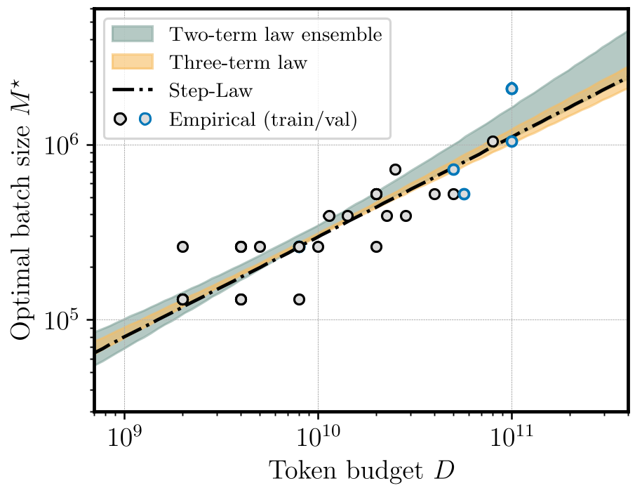Figure 1: The implied scaling of the optimal batch size (Right) shows that the 3-term law (solid line) perfectly tracks the empirically best batch sizes.

Experiments: Compute Savings of 72%

The most striking result is the efficiency of the fitting process. Traditionally, to find the optimal batch size scaling, you’d need a full sweep (5-10 batch sizes) for every point.

The authors show that with the 3-term law, you only need two batch sizes per configuration. Because the law understands the relationship between $M$ and $K$, it can "triangulate" the optimum from just a few points.

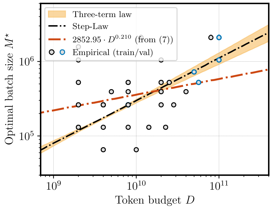Figure 2: Comparison of direct fitting vs. the Three-Term Law on reduced datasets. The 3TL (top row) remains stable even with 42% of the data, while direct fits (bottom) collapse.

Key Insight: The 5% Wasted Compute Rule

Practical hardware often prevents us from using the "mathematically optimal" batch size. The paper derives an interval $[b_{min},b_{max}]$ called the $ϵ$-suboptimal zone.

• Within this range, you waste less than 5% of your total compute.
• Rule of Thumb: This efficiency "plateau" typically has a width of about a factor of 4 (from $0.5imes$ to $2imes$ the optimal batch size).

Critical Analysis & Limitations

While the law is a massive step forward, it isn't perfect:

1. The Irreducible Loss Caveat: On some datasets (like Li), the fitted irreducible loss $E$ hits zero, which is theoretically impossible for natural language. This suggests the law is slightly under-parameterized for certain model-size effects.
2. Optimizer Sensitivity: The coefficients $(\beta ,\gamma )$ are likely tied to the AdamW optimizer. If the industry shifts to Muon or Soap, these laws will need re-calibration.

Conclusion (Takeaway)

The Three-Term Law bridges the gap between the "Chinchilla" obsession with quantity and the optimization theorist’s obsession with dynamics. For practitioners, it provides a blueprint to stop wasting compute on exhaustive sweeps and start using "suboptimal" data to find the optimal path.