
Making State Prediction Separation Almost Free: The Cost Case for a Cacheless Pause Query
Almost Free State Prediction Separation
This paper turns state-prediction separation into a free pause token by giving the prediction stream its own weight-shared forward computation without keys, values, or a sequence position. On a 1B Transformer, the method lowers next-token cross entropy by 0.0284 nats versus a matched control, and four cost controls reduce the overhead to 1.33 times wall clock while recovering about 94 percent of the gain, with a 1.09 times option that retains a smaller gain.
TL;DR
State-prediction separation improves next-token prediction by giving context summarization and token prediction separate streams, but the original form costs roughly 1.9 times the FLOPs of a standard Transformer. This paper pushes the idea to its limit with a free pause token: the prediction stream has no keys, no values, and no sequence position, so inference remains cacheless and step count remains unchanged. On a 1B parameter model trained on Phi-4 derived data, the full pause reduces cross entropy from 2.8957 nats to 2.8673 nats at 100B tokens, and a 42.5 percent phase start recovers about 94 percent of that gain at 1.33 times wall clock. The contribution is less a new modeling hypothesis than a rigorous cost accounting exercise showing when separation can become almost free.
Background and Positioning
This work sits at the intersection of architectural method and pretraining systems engineering. It inherits the state-prediction separation hypothesis from Monea and others and the idea of extra learned positions from pause-token research, but its novelty is in making the separation viable under wall-clock, memory, kernel compatibility, and isocompute constraints. That places it closer to compute-frontier engineering than to a pure scaling-law paper. The abstract frames the result as an isoflop, isoparameter, and isotoken improvement over standard next-token Transformers, but the paper itself shows that the improvement is real only after careful accounting: the strict iso-FLOP comparison narrows margins, and the best gains appear at wall-clock node-hours with phased training.
Problem and Motivation
A causal decoder predicts the next token from one hidden state per position. That state is asked to do two jobs simultaneously: summarize the prefix for future positions and be a good predictor for the immediate next token. The tension is not cosmetic. Later positions reuse the state as memory, while the LM head wants the same vector to be sharply predictive. State-prediction separation resolves this by running a second weight-shared prediction stream over the same backbone, but the solution is expensive because the second stream normally writes its own intermediate representation and often pays for additional attention bookkeeping.
The cost is twofold. At pretraining, a full second pass over layers can raise FLOPs to roughly 1.9 times the standard model. At inference, if the prediction stream becomes an actual extra sequence position, it expands context length, KV cache, and decode steps. The original pause-token idea adds learned non-vocabulary positions, which buys extra computation but spends sequence length. The practical question, therefore, is not merely whether separation lowers loss; it is whether separation can be implemented without making the older architecture with more tokens the better choice.
Core Method: From an Expensive Second Pass to a Free Pause
The starting point: why a raw second stream is not free
The paper's cost anchor is that a naive prediction stream reruns the Transformer layer stack but does not recompute the state's key and value projections. That yields an overhead close to, but below, exactly two times the standard FLOPs:
Here is the FLOPs cost of the unoptimized separated forward pass, is the FLOPs cost of a standard Transformer, and the factor 1.9 comes from the fact that the prediction pass reuses the state's keys and values rather than paying for a completely new projection pipeline. The important subtlety is that FLOPs are only part of the story. The paper notes that wall-clock time can be larger in practice because a flexible mask expressive enough to interleave state and prediction streams does not map cleanly to modern fused attention kernels. This is a systems bottleneck, not just a mathematical one. If the control model receives 1.9 times more compute at true iso-FLOP, the advantage of the full pause can shrink enough to become slightly negative, as the iso-FLOP discussion in Section 6.3 states: the phased deltas roughly halve and the full pause turns positive by about 0.006 nats. The method is therefore useful only if the second pass can be made much cheaper in wall-clock terms.
The core mechanism: a prediction query that leaves no cache
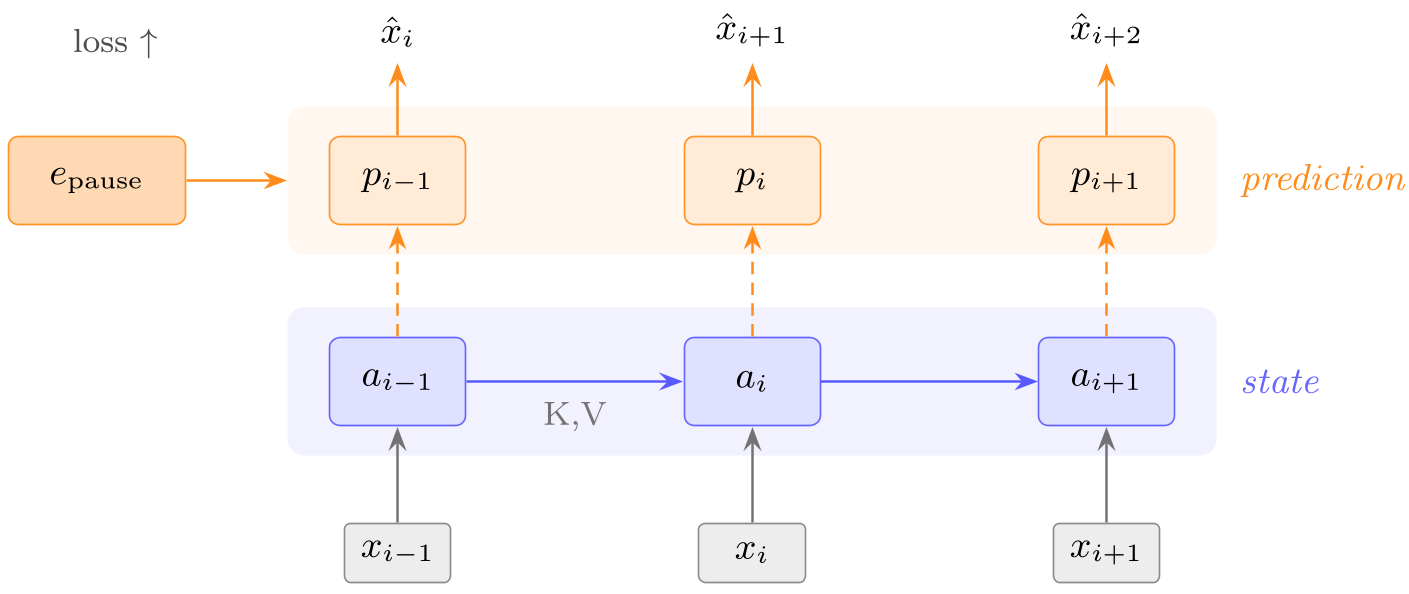
The free pause keeps the two-stream idea but removes the one feature that makes the second stream costly and disruptive: its write path. The state stream embeds tokens and produces persistent keys and values. The prediction stream starts from a single learned predict_embedding, forms a query at each layer, attends to the state's keys and values, and feeds the LM head. It writes nothing of its own:
The notation means that the prediction stream has no stored keys or values, and are empty, while its query reads only the state stream's keys and values up to position . This strictness is the paper's key insight. If the prediction stream wrote even temporary keys and values, it would still pollute the sequence's cache structure; if it occupied a new token position, it would expand context and decode cost. By writing nothing, the prediction stream becomes a shadow computation riding on existing positions. Because all backbone parameters are shared and only one additional learned embedding is inserted, the model is nearly iso-parameter, so a standard checkpoint remains a valid backbone. That property is what later enables phasing: the separation can be turned on only for the tail of training rather than paid across the entire run.
The cost controls: kernels, gates, windows, and schedules
The method's practicality rests on four mechanisms, and each trades quality or complexity against wall-clock cost. Table 1 in the paper summarizes them:
| Change | Cost effect | Quality effect |
|---|---|---|
| FlashAttention friendly split | Two separate passes run at 73k versus 16k tokens per second per GPU, about 4 times faster than a flexible interleaved mask | No quality loss reported |
| w=0 prediction window | Avoids the second log-sum-exp merged attention call, which costs 1.22 times the w=0 pass | Costs at most 0.009 nats, with 0.0047 nats measured at 100B |
| Shared gated FFN | Reduces full pause wall clock from 1.57 to 1.35 | Costs about 0.005 to 0.010 nats |
| Phasing at 42.5 percent | Reduces full pause wall clock from 1.57 to 1.33 | 2.8691 versus 2.8673 for full pause |
The first mechanism is not a mathematical trick but an execution strategy. Training is split into a state pass followed by a prediction pass that is plain cross-attention. This lets stock FlashAttention kernels express the computation directly. The second mechanism removes the prediction stream's own attention window. The paper finds that a small prediction self-window helps by only 0.0047 nats at 100B tokens, and Appendix B reports pause w=64 reaching 2.8626 versus w=0 at 2.8673. That is a clear quality-versus-engineering tradeoff: keeping the window would require a second merged attention call, so the authors accept the small loss and make the prediction strictly read-only over the archive.
The shared gated FFN is the most interesting design because it targets the dominant parameter mass of modern LLMs. Let and be the post-normalization residuals entering the FFN sub-layer. A single scalar gate mixes them, one FFN is evaluated, and two output gates route the result back:
In this expression, is a token-level scalar in the unit interval, is the sigmoid, and , are the small gating projections, and and are the outputs returned to the residual streams for state and prediction. The role of the equation is computational: one position-wise FFN evaluation replaces two. The boundary condition matters too. The gates are zero-initialized, which means every gate starts at 0.5, so the model does not need backbone parameter changes before phasing can begin. However, the switch is not exactly function-preserving. At initialization the sub-layer adds a single mixed FFN output to both streams, rather than applying separate FFNs to state and prediction, so training is required to settle. The paper measures the cost of this compromise as roughly 0.005 to 0.010 nats in full pause, a small price for removing stored second-pass FFN activations and increasing the feasible micro-batch.
Phasing then exploits the iso-parameter property. Standard training proceeds for a fraction of the schedule, then the split runs for the remainder:
The formula assumes the full split pays 1.57 times wall clock relative to the strong baseline; is the fraction trained as a standard Transformer and is the fraction trained with the second pass. For , the predicted overhead is 1.33 times; for , it is 1.14 times. This is the cleanest argument in the paper: because a standard checkpoint is already a valid backbone, the separation can be added late. The authors observe that a cold start with the full pause is actually worse for roughly 1.5B tokens, then becomes beneficial, which supports the intuition that early pretraining wants a simpler stable optimization path while later fine-grained separation can be more efficient.
Experimental Evidence and Compute Accounting
Main result at 100B tokens
The architecture is a 1B decoder with 24 layers, hidden size 1536, grouped-query attention with 16 query heads and 8 key-value heads, sliding-window attention of width 2048 on most layers, a full-attention layer every six layers, QK normalization, partial rotary embeddings on full-attention layers, tied embeddings, and sequence length 8192. Training uses Phi-4 derived data, global batch 524,288 tokens, Muon-family optimization with peak learning rate 2e-2, a warmup-stable-cooldown schedule with a final 25 percent cooldown to 2e-3, bf16 activations, and mxfp8 matrix multiplications on 8 B200 GPUs.
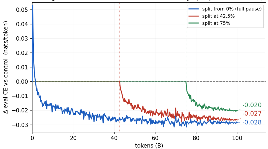
Table 2 reports the central iso-token result:
| Schedule | CE at 100B | Wall clock | Gain relative to full pause |
|---|---|---|---|
| control, no pause | 2.8957 | 1.00 | reference |
| full pause, w=0 | 2.8673 | 1.57 | reference |
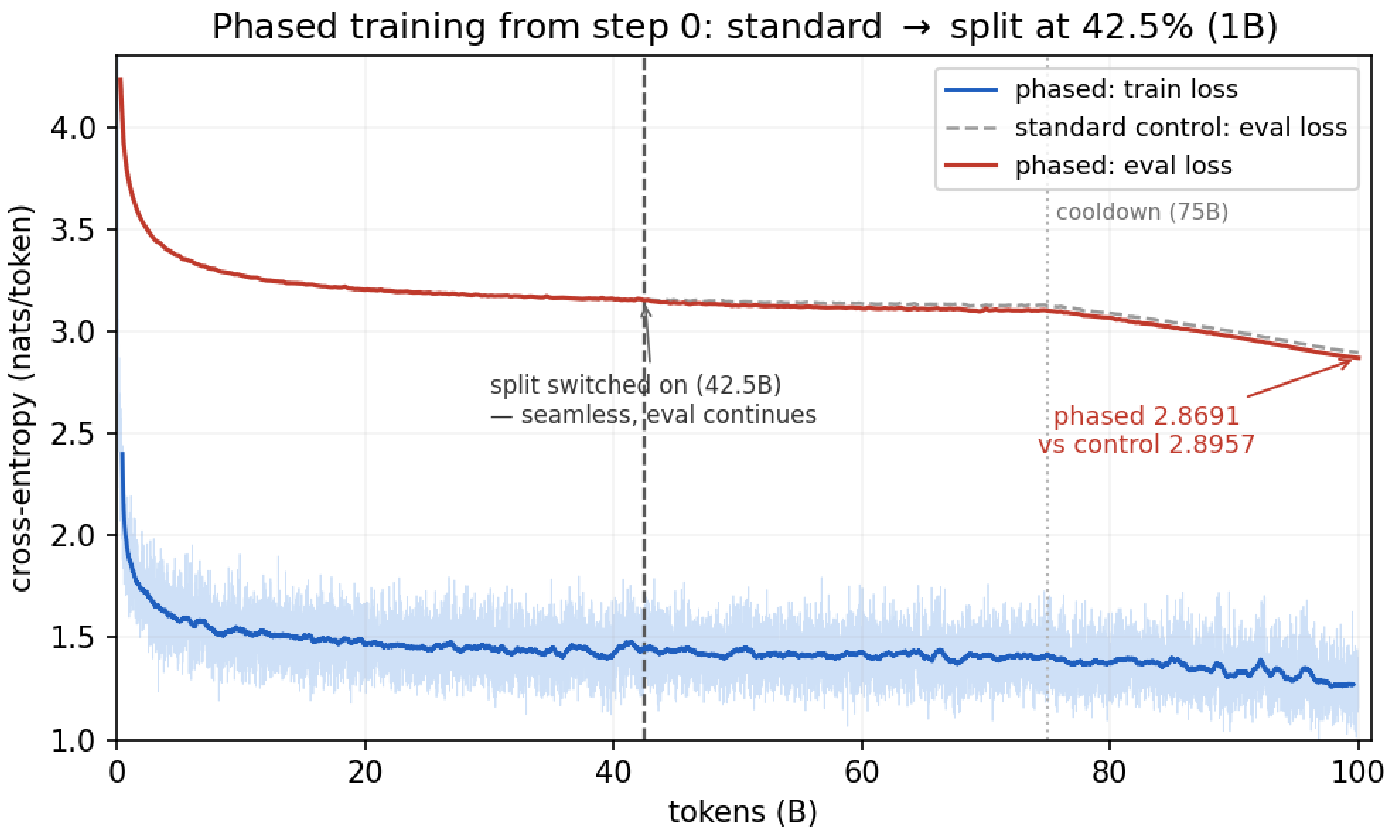
| 42.5 percent standard then pause | 2.8691 | 1.33 | 0.0018 behind, recovers 94 percent |
| 75 percent standard then pause | 2.8756 | 1.14 | 0.0083 behind, recovers 71 percent |
The main quality gain is small in absolute loss terms, 0.0284 nats, but meaningful in the pretraining economy where fractional nats are hard-won and inherited by downstream training. The important conclusion is not that the full pause is free, but that phasing makes most of the benefit almost free. The 42.5 percent phase point preserves nearly all of the quality at 24 percent of the full split cost, and the 75 percent point remains better than the control while costing only 1.14 times wall clock. Figure 3 reinforces the training-dynamics claim: the phased run tracks the standard control until the switch, then falls below it without a visible loss spike.
Shared FFN as the throughput frontier
Table 3 isolates the shared gated FFN under the faster micro-batch operating point. Because this changes the control as well, the paper compares against the matched shared-batch control:
| Shared gated FFN schedule | CE at 100B | Change versus control | Wall clock |
|---|---|---|---|
| control, no pause | 2.9064 | reference | 1.00 |
| full pause, w=0 | 2.8825 | 0.0239 lower | 1.35 |
| 42.5 percent standard then pause | 2.8886 | 0.0178 lower | 1.20 |
| 75 percent standard then pause | 2.8966 | 0.0098 lower | 1.09 |
The interpretation should be read carefully. Compared with Table 2, the control CE rises from 2.8957 to 2.9064 because the shared-FFN run uses a faster micro-batch operating point. The shared FFN therefore has two separate consequences: it slightly reduces quality relative to the two-pass free pause, and it changes the throughput frontier. The measured effect is that the shared form removes the second pass's stored FFN activations, freeing about 14 GB per GPU at peak memory, 91 GB versus 105 GB at micro-batch 4, and allowing a larger micro-batch. Throughput improves to 0.74 times the control, versus 0.64 times for the two-pass form. This is where the 1.09 times point comes from: shared FFN plus 75 percent phasing yields 0.0098 lower CE than the matched control. That is the paper's cheapest reported positive point.
Iso-compute and downstream capability
The paper's strongest claim is that the method survives equal node-hours. Table 4 uses the control's measured endpoints at 100B and 150B and an estimated slope of 0.037 nats per doubling:
| Variant | CE at 100B | Wall clock | Control at equal node-hours | Delta |
|---|---|---|---|---|
| full pause, w=0 | 2.8673 | 1.57 | 2.872 at 157B | 0.005 lower |
| 42.5 percent standard then pause | 2.8691 | 1.33 | 2.881 at 133B | 0.012 lower |
| 75 percent standard then pause | 2.8756 | 1.14 | 2.889 at 114B | 0.013 lower |
This table is the heart of the cost argument. If compute is counted only by tokens, the full pause appears best. If compute is counted by wall-clock node-hours, the cheaper phased variants can win more because the saved compute can be spent on extra control tokens. The caveat is that the 157B control endpoint is a short extrapolation, and a stricter iso-FLOP analysis tightens margins. The authors acknowledge this and still conclude that late-phase free pause training is a clear compute win of roughly one centinat depending on measurement convention.
Downstream evaluation supports the loss result. Table 5 reports DCLM CORE and climbmix bits-per-byte:
| Variant | DCLM CORE | climbmix BPB |
|---|---|---|
| control, 100B | 0.327 | 0.777 |
| control, 150B | 0.348 | 0.770 |
| full pause, w=0, 100B | 0.347 | 0.769 |
| 42.5 percent then pause, 100B | 0.348 | 0.769 |
| 75 percent then pause, 100B | 0.348 | 0.771 |
The numbers are modest but coherent. At iso-token, full pause raises DCLM CORE from 0.327 to 0.347 and lowers BPB by 0.008. At iso-compute, the 100B pause roughly matches the 150B control, and phased runs reach the same level for far less compute. The paper also notes that individual lm-eval task scores are inside their 95 percent intervals, so the evidence is pooled rather than task-specific. This is a useful honesty signal: the gain is real at dense aggregate measures, but it is not large enough to resolve cleanly on single 1B-scale tasks.
Inference cost and the embedding's role
Inference is where the design pays off directly. Prefill still forwards only ; no prediction is required and no prediction keys or values are written. At decode, state and prediction forward together as a two-token step that shares the KV read, so there is no additional sequence depth. Section 6.4 and Appendix A report a fused vLLM implementation where the decode step is within about 1 percent of a standard decode on B200 in a microbench. That claim is specific: it is not that inference is mathematically identical, but that the dominant latency terms, context growth, cache growth, and sequential decode steps, are unchanged.
The learned pause embedding itself is also interesting. Section 6.6 reports that it grows roughly 40 times from initialization to per-coordinate RMS near 1, but because it is RMS normalized before use, only its direction matters. That direction leans toward common continuations such as comma, period, newline, the, and and, with cosine similarities from 0.25 to 0.46. A few coordinates carry large spikes, about 11 percent of the energy in the top ten dimensions. Against the token-embedding table, it is atypical: near-orthogonal to the embeddings' common mode with cosine 0.05 and low norm relative to used tokens. This suggests the pause embedding is not merely another fake token; it is a specialized query vector that asks the backbone to turn its summarized state into a prediction without pretending to be another token.
Design Reasoning, Evidence Quality, and Limitations
The most defensible part of the paper is its accounting discipline. It does not simply compare loss curves. It compares optimized wall-clock throughput, reports the 20 percent utilization advantage of the compute-dense second pass, uses matched controls at global batch 524,288, converts the cost from raw FLOPs to node-hours, and then re-tests at iso-FLOP. That layering is what makes the result credible: small pretraining wins can vanish if extra compute is handed to the baseline, and the authors explicitly show where that happens.
The evidence is strongest for the 42.5 percent phased pause. Table 2 shows it recovers 94 percent of the full pause gain at 1.33 times wall clock, and Table 4 shows a 0.012 nat iso-node-hours advantage. The shared FFN frontier is also strong because it moves the cheap end of the tradeoff to 1.09 times wall clock while still beating its matched control by 0.0098 nats. The weakest part is generality. The paper states that experiments are limited to a single scale of 1B with a single primary seed, although it argues pretraining is robust enough that the effects are above noise. That argument may be reasonable for large, well-matched controls, but it does not establish scaling behavior.
A second limitation is that some cost claims rest on measured throughput plus extrapolation. Table 4's control endpoints at 114B, 133B, and 157B are interpolated or short extrapolated from measured 100B and 150B endpoints using a loss slope of 0.037 nats per doubling. This is plausible, but it means the iso-compute margin of 0.005 to 0.013 nats depends on the local scaling law. The authors partially guard against this with the stricter iso-FLOP note, where the full pause becomes slightly negative. That caveat should not be buried; it says the method's advantage is schedule-sensitive, not universal.
A third limitation is architectural narrowness. The experiments use a specific 1B configuration with sliding window 2048, periodic full attention, QK normalization, partial rotary, Muon, Phi-4 data, and an 8192 sequence. The method's key requirements are clear: the prediction stream must remain query-only, the FFN gate must learn to route, and phase switching must be stable. But the paper does not provide formal proofs or multi-scale phase point recommendations. It does not report whether 42.5 percent or 75 percent remains optimal at 7B or larger models, at different sequence lengths, or on data with different entropy.
Insights and Future Directions
The deeper lesson is that the free pause is a way of spending inference-time compute without spending sequence structure. It occupies the same computational niche as speculative decoding and multi-token prediction: extra forward work can be useful if it can be fused with existing memory accesses. But this paper repurposes that intuition for prediction quality at training and inference, not token speed. The separation works because the state stream can specialize as memory and the prediction stream can specialize as query, and it remains cheap only if the prediction stream leaves the cache topology untouched.
A natural next step is to evaluate free pause separation at multiple seeds and model scales, especially because phasing relies on the convex quality-versus-node-hours curve seen in Figure 1. Another is to combine it with speculative decoding or multi-token prediction, since both exploit similar spare compute. The paper itself points to multi-token prediction as a potentially significant variation, but does not test it. A third direction is automatic phase point selection. The current evidence suggests that a late phase, 42.5 to 75 percent, is where much of the value lies, but the best point likely depends on total budget, sequence length, and optimizer state stability. Finally, the shared gated FFN should be studied as a reusable primitive: it is essentially a cheap way to fuse two residual streams when one stream is query-like and the other is state-like, and that pattern may appear beyond pause-token prediction.