
Deep Autoencoders: Reimagining Gene Ontology Annotation as Matrix Completion
Deep autoencoder neural networks for gene ontology annotation predictions
This paper introduces deep autoencoder neural networks for Gene Ontology (GO) annotation prediction, framing the task as a matrix-completion problem. The method outperforms several established baselines, including Truncated Singular Value Decomposition (tSVD), pLSA, and LDA, on multiple biological datasets.
TL;DR
Gene functional annotation is the backbone of modern bioinformatics, yet our current databases are "Swiss cheese"—full of holes and inaccuracies. This paper demonstrates that Deep Autoencoders can treat gene annotation as a non-linear matrix completion problem, significantly outperforming traditional linear methods like SVD and probabilistic models like LDA. By leveraging deep architectures, the authors achieved up to a 36% improvement in predicting new annotations for cattle and red junglefowl genomes.
Background: The Annotation Gap
The Gene Ontology (GO) project maps genes to functional features across three domains: Biological Processes, Cellular Components, and Molecular Functions. However, as of this paper's publication, thousands of annotations were still missing. Traditional computational aids relied heavily on Truncated Singular Value Decomposition (tSVD)—a technique that finds the "best linear fit" for a data matrix.
The core insight of this work is that biological relationships are rarely just linear. If a gene is involved in "DNA binding," its secondary and tertiary functional associations aren't just simple correlations; they are complex, hierarchical dependencies that require the expressive power of Deep Learning.
Methodology: From Linear SVD to Non-Linear Autoencoders
The authors treat the GO database as a binary matrix , where rows are genes and columns are GO terms.
1. Annotation Unfolding
Before feeding data into the model, they perform "unfolding." Since the GO is a Directed Acyclic Graph (DAG), if a gene is annotated with a specific child term, it is implicitly annotated with all its parents. This process ensures the model sees a logically consistent snapshot of biology.
2. The Autoencoder Architecture
An autoencoder is a neural network designed to reconstruct its input. The "magic" happens in the hidden layers:
- The Bottleneck: By having fewer units in the hidden layers than the input, the network is forced to learn a compressed, "latent" representation of gene functions.
- Non-linearity: Unlike tSVD (which is essentially a linear autoencoder), this model uses Sigmoid activation functions. This allows the model to capture "XOR" style relationships and complex logical dependencies between different GO terms.
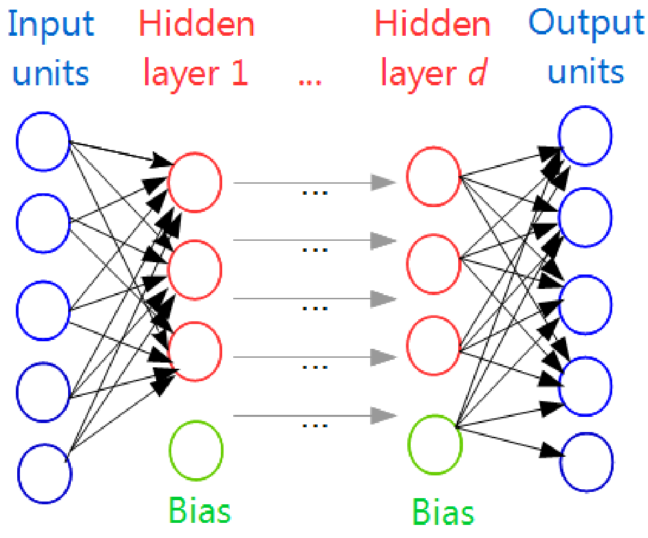 Figure 1: A multi-layer autoencoder. The input gene profile is compressed and then reconstructed, with the output effectively serving as a "cleaned" and "completed" version of the original annotation.
Experiments and SOTA Comparison
The authors tested their approach on six datasets (two species, three sub-ontologies). They used 2009 data for training and 2013 data to see if the model could "predict the future"—i.e., identify annotations that biologists would eventually discover and add to the database manually.
Performance Metrics
The performance was measured by checking how many of the "top 100" model predictions actually appeared in the database updates between 2009 and 2013 (the upDB% metric).
| Dataset | tSVD | pLSA | Autoencoder (AE) | Improvement |
|---|---|---|---|---|
| Bos taurus (BP) | 14% | 30% | 45% | +15% |
| Gallus gallus (MF) | 6% | 16% | 52% | +36% |
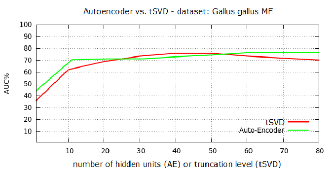 Figure 2: Hyper-parameter analysis showing that the Autoencoder (red) consistently maintains higher AUC values across different model complexities compared to linear tSVD (blue).
Critical Insight: Why Does It Work?
The superiority of the autoencoder stems from its Inductive Bias. While tSVD forces the data into a rigid k-dimensional subspace, the deep autoencoder learns a manifold—a curved "surface" in high-dimensional space where real gene functions actually reside.
The results in Table 3 show a massive leap in Molecular Function (MF) prediction for the Gallus gallus dataset (an improvement from 16% to 52%). This suggests that MF annotations might contain the specific type of complex, non-linear dependencies that linear models simply cannot see.
Conclusion and Future Outlook
This work marks a shift from classical matrix factorization to deep generative modeling in genomics. By treating the Gene Ontology as a compressed sensing problem, the authors provided a tool that doesn't just catalog known biology but actively points researchers toward the next discovery.
Takeaway for the Industry: The success of autoencoders here foreshadows the shift toward using Latent Space representations for drug discovery and functional genomics. While modern researchers might now use Graph Neural Networks or Transformers for this task, the transition from linear to non-linear "bottleneck" models was the critical turning point established by works like this.