MLRSS: Bridging Machine Learning and Geostatistics for Environmental Risk Mapping

TL;DR

This seminal work addresses the challenge of modeling highly non-stationary environmental data, such as the 137Cs fallout from the Chernobyl disaster. The authors propose the MLRSS (Machine Learning Residuals Sequential Simulation) framework, a hybrid model that utilizes Multilayer Perceptrons (MLP) and Support Vector Regression (SVR) to capture complex global trends, while employing Geostatistical Sequential Gaussian Simulations (SGS) to handle local stochastic variability and uncertainty.

The Problem: When Stationarity Fails

In environmental science, we often assume that data is "stationary"—meaning its statistical properties don't change across space. However, real-world catastrophes like radioactive leaks or pollutant spills create non-linear spatial trends and "spotty" patterns that traditional Kriging cannot handle.

Current geostatistical tools like Universal Kriging attempt to solve this using polynomial trend models, but these are often too simple. The core challenge is: how do we extract a complex, deterministic trend without over-fitting the noise, while still maintaining a robust measure of uncertainty?

Methodology: The "Detrending" Pipeline

The authors decompose the spatial process $Z(x)$ into two components: $Z(x)=M(x)+e(x)$ Where $M(x)$ is the large-scale deterministic trend and $e(x)$ is the small-scale stochastic residual.

1. The ML Trend Extractor

The paper evaluates two heavyweights of the era:

• Multilayer Perceptron (MLP): Uses backpropagation to find non-linear patterns. The authors found that a single hidden layer with just five neurons was optimal for capturing the trend without "learning the noise."
• Support Vector Regression (SVR): Leverages the Statistical Learning Theory (SLT) and the $\epsilon$-insensitive loss function. By using a Radial Basis Function (RBF) kernel, SVR provides a robust, sparse solution for spatial regression.

2. Geostatistical Residual Modeling

Once the ML model predicts the trend, the residuals (the difference between actual and predicted) are transformed into a normal score distribution. Geostatistical tools (variography) are used to analyze the remaining spatial correlation. Finally, Sequential Gaussian Simulation (SGS) generates hundreds of equiprobable "realizations" of these residuals.

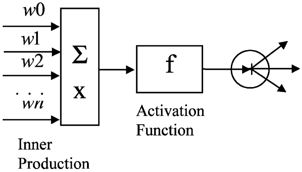Fig 1: The architecture of the MLP used to extract non-linear environmental trends.

Experiments & Results: The Chernobyl Case Study

The researchers applied this to a 7,428 km² area contaminated by 137Cs.

• Trend Extraction: Both MLP and SVR successfully identified the high-concentration zones near the source.
• Residual Analysis: The residuals showed significant spatial correlation (correlation coefficients of ~0.78), validating that the ML models captured the global trend while leaving the structured local variability for geostatistics to solve.
• Risk Mapping: The ultimate goal was Probabilistic Mapping. Unlike deterministic estimates, the hybrid model allows decision-makers to see the probability of contamination exceeding a safety threshold (e.g., 800 kBq/m²).

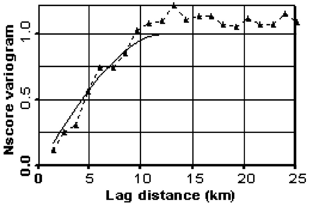Fig 2: SVR trend modeling showing the large-scale spatial distribution of contamination.

Critical Insight: Why Hybridize?

The genius of this approach lies in the division of labor:

1. ML is the Globalist: It excels at finding non-linear, high-dimensional functions (the "Why" of the trend) based purely on data.
2. Geostatistics is the Localist: It excels at characterizing the "Uncertainty." It understands that nearby points are related and provides a probabilistic framework that "black-box" ML often lacks.

Limitations

• Expert Knowledge required: The framework isn't a "push-button" solution; it requires deep expertise in variography and hyperparameter tuning for the ML models.
• Clustering Sensitivity: Like most spatial models, the performance is highly dependent on the representativity of the sampling points.

Conclusion & Future Outlook

The MLRSS model represents a significant leap from traditional "Kriging with a trend." By integrating the flexibility of ML with the statistical rigor of geostatistics, the authors provided a powerful tool for environmental risk management. For modern practitioners, this work serves as an early blueprint for current Physics-Informed Neural Networks (PINNs) and Gaussian Process hybrids used in environmental AI.