Collaborative Intelligence: Mobile Sensor Networks for Autonomous Field Estimation

    ## TL;DR
    How can a swarm of mobile robots map an unknown environmental field—like a spreading oil spill or air pollution—without a central brain? This paper proposes a dual-algorithm approach: **Distributed Support Vector Regression (SVR)** for learning the field function and **Lloyd’s CVTs** for intelligent deployment. The result is a self-organizing network that autonomously clusters where the action (or pollution) is highest.

    ## The Challenge: Mapping the Unknown with Local Data
    In environmental monitoring, we often face a "chicken and egg" problem. To deploy sensors efficiently, you need to know where the field (e.g., chemical concentration) is highest. But to find those high-concentration zones, you need sensors deployed there first. 

    Prior works either assumed the field was known a priori or relied on complex communication paths (like Gaussian elimination across the whole network) that fail when robots are moving or out of range. The core motivation here is to build a system where robots talk only to their immediate neighbors but still converge on a global understanding of the environment.

    ## Methodology: The "Bump" Kernel & Adaptive Coverage
    The authors break the task into two interlocking loops:

    ### 1. Learning with Localized SVR
    Traditional SVR find a function $f(q)$ that fits sensor readings. The "secret sauce" here is a **Kernel with Finite Support**. 
    By using a "bump function" that drops to zero beyond a distance $B$, the authors ensure that a sensor node only needs to consider its neighbors to update its prediction.
    
    ![Algorithm Flow](https://cdn.atominnolab.com/wisdoc/formulas/20260606-25e38295-986d-4c41-9efa-3ee9e2e218a9/page_002_block_002.png)
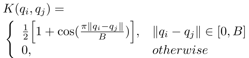
    *The Finite Support Kernel: Crucial for making global regression a local computation.*

    ### 2. Moving with Lloyd's Algorithm
    Once a robot has a local estimate of the field $f(q)$, it treats that function as a **density map**. Using Centroidal Voronoi Tessellations (CVT), each node calculates its Voronoi region and moves toward the "center of mass." Since the mass is weighted by $f(q)$, the nodes naturally drift toward regions with higher values (the peaks).

    ## Putting it to the Test: Simulation Results
    The framework was validated in two challenging scenarios with a 30-node network:

    - **Static Fields**: The network successfully identified three distinct Gaussian peaks. As shown in the error curves, the cumulative error drops sharply and plateaus once the sensors reach an optimal distribution.
    - **Dynamic Fields**: The most impressive part of the study involves moving peaks. Even as the "pollution" sources drifted across the map at different speeds, the swarm reshaped its formation to track them in real-time.

    ![Dynamic Tracking Results](https://cdn.atominnolab.com/wisdoc/images/20260606-25e38295-986d-4c41-9efa-3ee9e2e218a9/page_004_block_004.png)
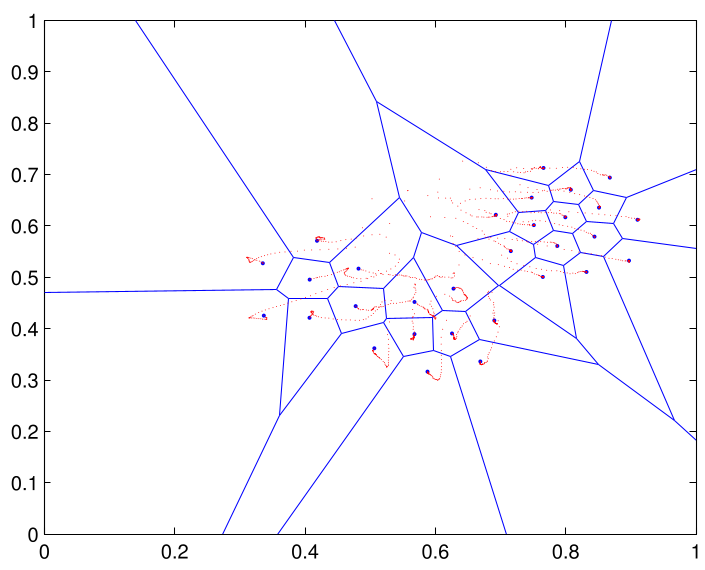
    *Visualizing the dynamic simulation: The left shows the ground truth, and the right shows the sensor network's real-time estimation as the peaks move.*

    ## Critical Analysis & Professional Insight
    The brilliance of this work lies in its **simplicity and locality**. By restricting the kernel support to the communication range, the authors effectively bypass the "curse of dimensionality" and the communication bottlenecks typically found in distributed optimization.

    **However, a few trade-offs remain:**
    - **Local Minima**: As noted by the authors, the network can get stuck in local minima if the initial distribution is too far from the actual peaks.
    - **Sparsity Error**: The "static error" seen in results is a function of node density. In real-world scenarios (like the SHOAL project with robotic fish), hardware costs might limit the number of nodes, making the choice of kernel bandwidth $B$ a critical hyperparameter.

    ## Conclusion: The Future of Robotic Swarms
    This paper demonstrates that distributed machine learning is not just for data centers—it is a powerful tool for physical world interaction. By marrying ε-SVR with CVT-based coverage, the researchers have created a robust, scalable system for monitoring harmful contaminants in ports and oceans. Future work involving "exploration behaviors" will hopefully allow these swarms to search even more aggressively for hidden leaks.

    ![Final Trajectories](https://cdn.atominnolab.com/wisdoc/images/20260606-25e38295-986d-4c41-9efa-3ee9e2e218a9/page_005_block_005.png)
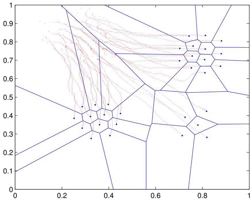
    *Trajectory of sensors: Notice how nodes converge toward high-value regions while maintaining space to ensure coverage.*