GIIM: Mastering the "Relationship Logic" of Clinical Diagnosis via Heterogeneous Graphs

TL;DR

Diagnosis is rarely about looking at a single image; it's about connecting the dots between different views and multiple lesions. GIIM (Graph-based Learning of Inter- and Intra-view Dependencies) is a new framework from NVIDIA researchers that treats a patient's case as a Heterogeneous Graph. By explicitly modeling how tumors evolve across time phases (Inter-view) and how they relate to neighboring abnormalities (Intra-view), GIIM sets a new SOTA for CT, MRI, and Mammography, even when crucial imaging data is missing.

Academic Standing: This work moves beyond simple "feature fusion" and introduces a flexible, relationship-aware topological structure that mimics a radiologist's holistic reasoning.

Problem & Motivation: The "Single-View" Blindness

In clinical practice, a radiologist doesn't just look at a "malignant-looking" spot. They ask:

1. Temporal/View Dynamics: How does this lesion look in the Arterial phase vs. the Delayed phase of a CT?
2. Spatial Context: Is this small lesion near a larger one? Certain tumor types tend to cluster or appear in specific patterns.

Existing CADx models—including standard CNNs and Transformers—often fail here because they typically require fixed-size inputs and treat lesions as independent samples. Furthermore, "Missing View" data (e.g., a patient missed a specific MRI sequence) often breaks traditional multi-view pipelines.

Methodology: The Core Architecture

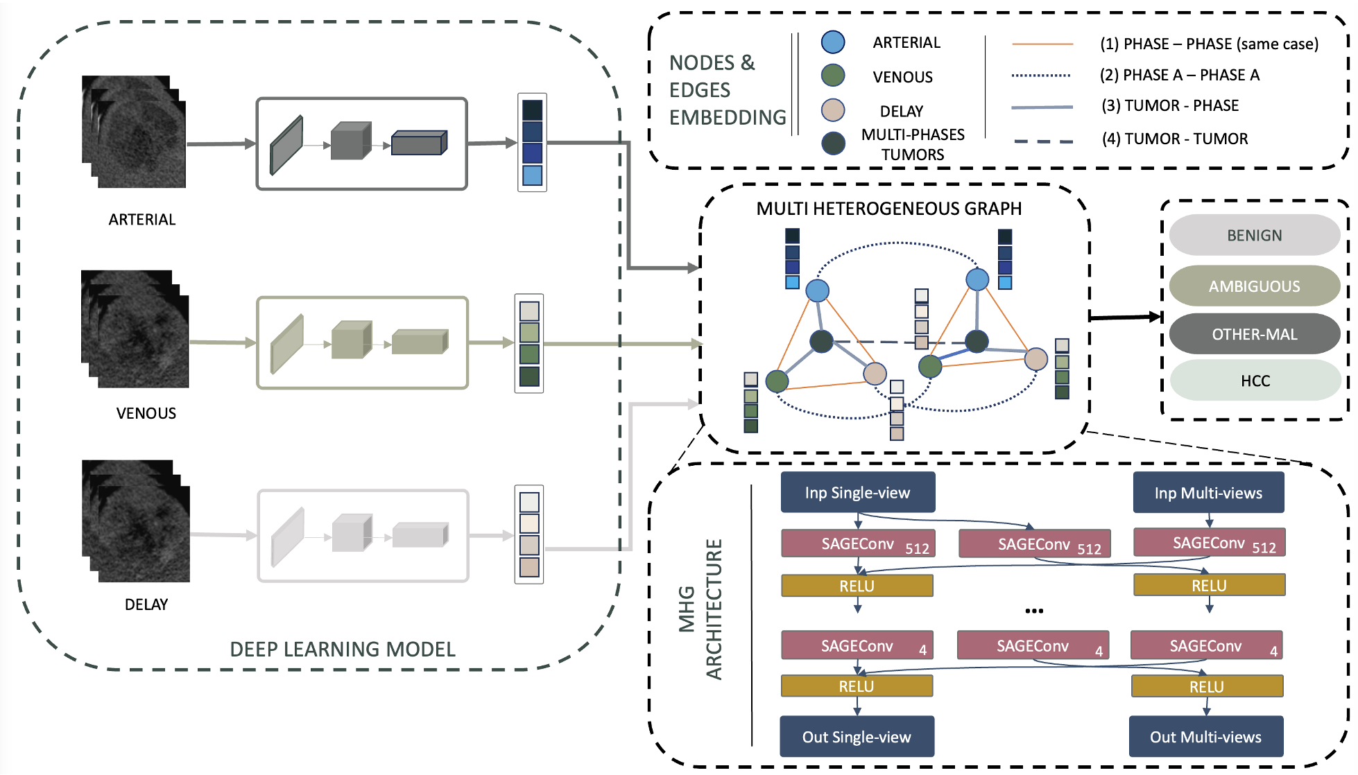
GIIM reframes diagnosis as a graph problem. Every patient case is converted into a Multi-Heterogeneous Graph (MHG).

1. The Global Architecture

The workflow starts with a ConvNeXt backbone (Stage 1) to extract "feature seeds." These seeds are then populated into a graph (Stage 2) where nodes and edges perform the heavy lifting of reasoning.

2. Modeling the Edge Logic

The "secret sauce" lies in the four types of edges defined by the authors:

• Intra-tumor, Inter-view ($E_{intra}$): Links different phases of the same lesion (Temporal tracking).
• Inter-tumor, Single-view ($E_{inter-s}$): Links different lesions in the same image (Spatial context).
• Single-to-Multi-view ($E_{s-m}$): Connects specific view nodes to a "summary" node of that lesion.
• Inter-tumor, Multi-view ($E_{inter-m}$): High-level contextual relationship between all abnormalities found in the patient.

3. Handling the "Missing Data" Crisis

GIIM doesn't just fail when a view is missing. The authors propose several imputation strategies:

• Covariance-based: Imputing missing features by finding statistically similar samples in a database using covariance metrics.
• RAG-based: Using a retrieval-augmented strategy to "borrow" features from the most similar complete case in the training set.

Experiments & Results: Proving Robustness

The researchers tested GIIM on three distinct challenges: Liver CT, Mammography (VinDr-Mammo), and Breast MRI.

SOTA Comparison

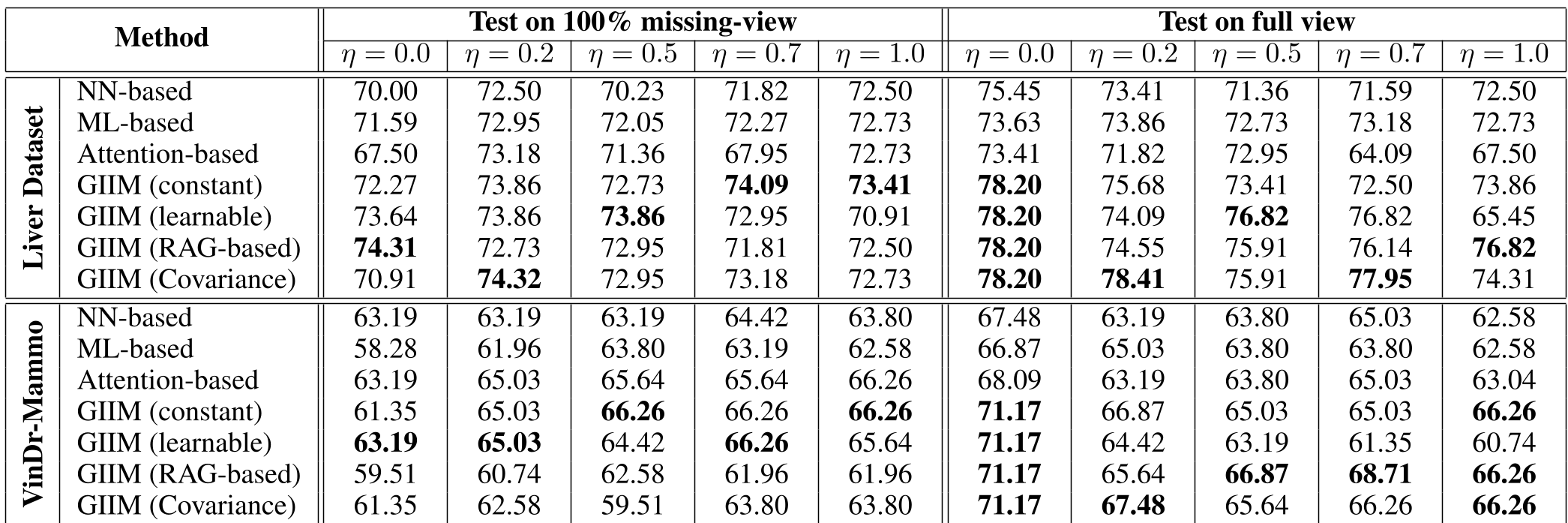
GIIM consistently outperformed Attention-based and ML-based (LightGBM) models. In the Liver Dataset, it achieved an AUC of 91.05%, a significant jump from the 82.78% achieved by single-view arterial scans.

The Missing Data Stress Test

Even when views were simulated as missing ($\eta$ ranging from 0.0 to 1.0), the GIIM (Covariance) and GIIM (Constant) models maintained higher accuracy than traditional Neural Networks. This proves that the graph structure allows the model to "fill in the blanks" using information from surviving nodes.

Critical Analysis & Conclusion

Takeaway

GIIM successfully demonstrates that Heterogeneous Graphs are a natural fit for medical imaging. Unlike Transformers, which have a global receptive field that can be "noisy," the graph structure imposes an inductive bias that matches clinical logic—specifically the connection between specific phases and related lesions.

Limitations & Future Work

While GIIM is powerful, it relies on a pre-trained backbone (ConvNeXt). If the initial feature extractor fails to capture a lesion, the graph cannot "reason" it back into existence. Future work might involve End-to-End Graph-Vision training where the graph gradients directly update the CNN weights to better capture relationship-relevant features.

Final Thought

For AI to be trusted in clinics, it must handle the "messiness" of real-world data. GIIM’s focus on missing-data robustness and inter-lesion context brings us one step closer to an AI that thinks like a Senior Radiologist.