HOPE: Deconstructing Deep Networks via Hilbert Functional Projection

TL;DR

Researchers from Google DeepMind and UC Berkeley have introduced HOPE (Hilbert Operator for Progressive Encoding), a mathematical framework that treats deep neural networks not as static matrices of weights, but as a collection of continuous functions in a Hilbert space. By shifting the perspective from "What is the weight magnitude?" to "What does this neuron actually do?", they've created a data-free, hyperparameter-free method for model compression and transfer learning that outperforms traditional heuristics like magnitude pruning and EWC.

The "Scale Symmetry" Trap: Why Magnitude is Deceptive

For years, the standard way to "clean" a network was Magnitude Pruning: if a weight is small, kill it. However, this is fundamentally flawed. Due to Batch Normalization (BN) and Positive Homogeneity (PH-1) in activations like ReLU, a network can scale its weights up or down without changing its output logic. Optimization artifacts often create "large" weights that are functionally useless or "small" weights that carry critical signals.

HOPE argues that we must analyze neurons in the Function Space. A neuron is defined by its end-to-end signal mapping, accounting for input weights, BN statistics, and output projections.

Methodology: Lifting Neurons into Hilbert Space

HOPE’s core innovation is modeling each neuron as a rank-1 Hilbert-Schmidt operator.

1. Gaussian Surrogates: Since we don't always have the original data, HOPE uses the Maximum Entropy Principle. It uses the BN statistics stored in the model to create a "proxy" input distribution.
2. Functional Inner Product: Instead of comparing weight vectors, it calculates the Kernel $K(i,j)$, which measures the expected alignment of two neurons' activations over the data manifold.
3. Unified Projection Cost: Whether pruning a neuron (projecting to zero), merging two neurons (projecting to a shared parent), or evicting a block, HOPE uses a single metric $J$. This metric measures the "distortion" in function space, normalized by the layer's surviving capacity.

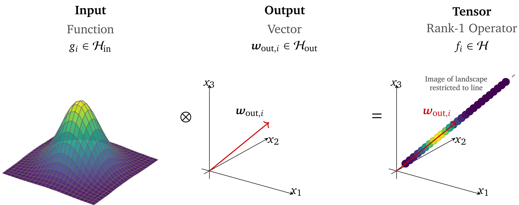Figure 1: Neurons are modeled as tensors where the infinite-dimensional input landscape is bound to a finite-dimensional output weight.

Pruning vs. Merging: The Geometry of Redundancy

A unique feature of HOPE is its ability to merge neurons. Overparameterized networks often "fragment" a single feature across many correlated neurons. Simple pruning would throw away information. HOPE uses a rank-2 to rank-1 projection—effectively "zipping" redundant neurons into a single, optimal parent that maintains the signal while freeing up parameter space.

Experiments: Performance and Stability

The authors tested HOPE on ResNet-50 and a transfer learning scenario dubbed DEFT (Dispersed Elastic Fine-Tuning).

1. Model Compression SOTA

Against standard structured pruning baselines, HOPE maintains higher accuracy as model density decreases. It avoids "catastrophic collapse" by accurately identifying functional foundations.

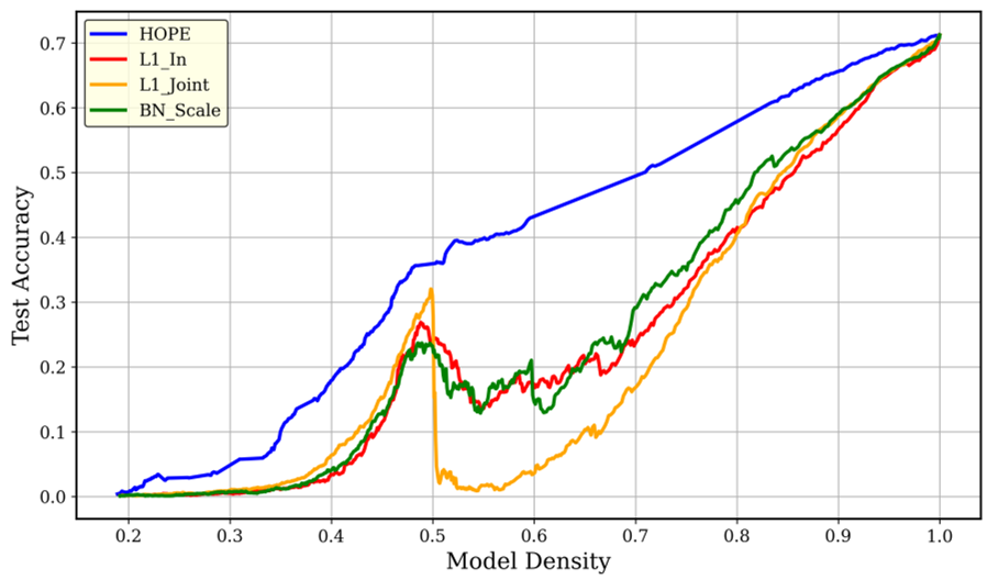Figure 2: HOPE maintains superior accuracy-density trade-offs compared to BN-scaling or L1-norm pruning.

2. Solving the Stability-Plasticity Dilemma

In transfer learning (e.g., CIFAR-100 to SVHN), models typically either forget the old task (Full FT) or fail to learn the new one (Head-only). DEFT uses HOPE to:

• Freeze the "Universal Core": High-capacity neurons are locked.
• Release the "Peripheral Slack": Low-capacity or redundant neurons are made plastic.
• Structural Masking: It severs connections from new "learning" neurons to the frozen core to prevent signal interference.

The result? An H-Score (harmonic mean of source and target accuracy) that is 5x higher than Elastic Weight Consolidation (EWC).

Critical Analysis & Conclusion

HOPE represents a significant shift toward principled architectural surgery. Its greatest strength is its data-free nature—it "interrogates" the network's own statistics to understand its identity.

Limitations:

• The Gaussian surrogate assumption, while theoretically supported by the Diaconis-Freedman effect, may struggle with highly non-Gaussian manifolds in very sparse, late-stage layers.
• Current implementation focuses on PH-1 activations (ReLU, Leaky ReLU); extending this to Swish or GeLU would require new kernel derivations.

Future Work: This framework opens the door to Automated Interpretability. If we can mathematically identify the "Universal Core," we might finally be able to isolate and label the fundamental concepts a model has truly mastered.