The Shannon Scaling Law: LLMs as Noisy Channels and the End of Monotonic Scaling

TL;DR

Scaling laws have long been the North Star of AI, but the "bigger is always better" mantra is hitting a wall. A new paper, LLMs as Noisy Channels, introduces the Shannon Scaling Law. By treating LLMs as communication channels, the authors replace simple power laws with information theory. This new law successfully models why performance sometimes drops as you scale (catastrophic overtraining/quantization) and accurately predicts model behavior even 1.7x beyond the training data limit.

Background Positioning

In the academic coordinate system, this work moves LLM theory from Empirical Observation (fitting curves to data) to Theoretical Grounding (applying Shannon’s Information Theory). While OpenAI’s original law and DeepSeek’s Chinchilla law work in "clean" regimes, they collapse under noise. This paper provides a unified theory for both standard pretraining and "messy" real-world scenarios like low-bit quantization and noisy fine-tuning.

1. The Death of Monotonicity: Why Scaling Breaks

The AI industry has been obsessed with the idea that $Loss\propto 1/Scale$. However, we are seeing more "U-shaped" performance curves:

1. Catastrophic Overtraining: Training too long on a specific task (SFT) can actually make the model worse.
2. Quantization Sensitivity: Larger models are sometimes more fragile when compressed to 2-bit or 3-bit.

Traditional laws can't see these "basins" of loss because they don't understand Noise. The authors argue that as you scale $N$ (Parameters) and $D$ (Tokens), you aren't just scaling knowledge—you are scaling the inherent noise of the system.

2. Methodology: From Hertz to Hyperparameters

The core innovation is mapping the Shannon-Hartley Theorem ($C=B\log (1+S/N)$) to LLM training dynamics:

• Bandwidth ($B$): Mapped to Model Size ($N$). A larger model has more "frequencies" to capture complex patterns.
• Signal ($S$): Mapped to Training Tokens ($D$). More data provides the signal to be transmitted into the weights.
• Noise ($\mathcal{N}$): Decomposed into Data noise (typos/errors), Model noise (random initialization/interference), and Irreducible noise (architectural limits).

The Math of Performance

The loss is defined as the reciprocal of this capacity: $\mathcal{L}(N,D)=\frac{1}{a{N}^{\alpha }{\log }_2\left(1+\frac{b{D}^{\beta }}{c(DN{)}^{\gamma }+d{D}^{\delta }+e}\right)}$

Figure: The structural correspondence between the Shannon communication model and LLMs.

3. The "Loss Basin" and Empirical Evidence

The researchers tested this on Pythia and OLMo2 across three "perturbation" types: Gaussian noise, SFT, and Quantization.

The Visualization of Scaling Failure

In the high-SNR (clean) regime, the loss landscape is open. But as noise increases, a "basin" forms. If you move too far left (too small) or too far right (overtrained), the loss shoots up.

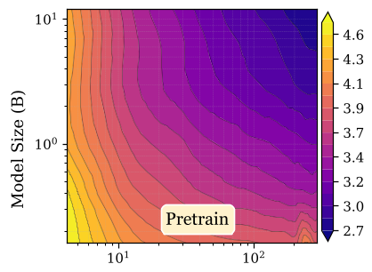Figure: Evolution of Pythia loss contours. Note the transition from monotonic improvement to U-shaped degradation at 10dB noise.

Results: Predictive Power

The most impressive feat is Extrapolation. Standard laws fail when asked to predict the performance of a model larger than any seen in the training set. The Shannon Scaling Law maintained an $R^2$ of 0.847 when predicting a 12B model from 6.9B data, while OpenAI and Chinchilla laws essentially collapsed.

4. Why This Works: The Exponent Inversion

The authors conducted an ablation study on the exponents ($\alpha ,\beta ,\gamma ,\delta$). They found a critical insight:

• In Low-SNR regimes, the Noise exponent ($\gamma$) grows faster than the Bandwidth exponent ($\alpha$).
• Conclusion: Scaling model size becomes detrimental because the noise amplification outpaces the information gain.

This explains the "Over-parameterization Paradox"—if your data signal isn't clean enough, a bigger model will just "memorize" the noise more efficiently, leading to worse generalization.

5. Critical Analysis & Future Outlook

Takeaways

• Stop Brute-Force Scaling: We are approaching a regime where data quality (SNR) is more important than raw token count.
• Strategic Training: This law helps practitioners find the "Sweet Spot"—the bottom of the loss basin—before degradation begins.

Limitations

• Constant Fitting: The law requires fitting 6-9 parameters, which may require several small-scale "pilot" runs (N x D grid) to identify the specific noise profile of a dataset.
• Architecture Specificity: While tested on Transformers (Pythia/OLMo2), it remains to be seen if modern architectures like Mamba or RWKV follow the exact same noise-interaction ($\gamma$) scaling.

The Shannon Scaling Law provides a much-needed theoretical rug to stand on as we push models into the trillion-parameter range where empirical observation alone is no longer enough to avoid catastrophic failure.