
[Finance & ML] Cracking the Low-Volatility Anomaly: Why "Low Risk" Is Just Different Risk
THE LOW-VOLATILITY ANOMALY AND THE ADAPTIVE MULTI-FACTOR MODEL
This paper introduces a novel explanation for the low-volatility anomaly using the Adaptive Multi-Factor (AMF) model estimated via the Groupwise Interpretable Basis Selection (GIBS) algorithm. By mapping portfolios to a high-dimensional set of ETF-based basis assets, the authors demonstrate that low-volatility stocks outperform because they load on specific, high-performing risk factors (like Bonds and Real Estate) rather than acting as an independent source of alpha.
Executive Summary
TL;DR: For decades, the "Low-Volatility Anomaly" has been the "ghost in the machine" for financial theorists—low-risk stocks consistently beat high-risk ones, defying the fundamental risk-reward trade-off. This paper provides a data-driven exorcism. By applying the Adaptive Multi-Factor (AMF) model and the GIBS algorithm, the authors prove that low-volatility stocks aren't "magical"; they simply represent a different set of underlying risk factors (like Bonds and Real Estate) that the traditional Fama-French 5-factor model is too rigid to see.
Positioning: This work is a SOTA methodological refinement. It bridges the gap between high-dimensional machine learning (clustering/LASSO) and classical Arbitrage Pricing Theory (APT), effectively "pricing" an anomaly that was previously thought to be a market inefficiency.
The "Anomaly" That Wouldn't Die
According to the Capital Asset Pricing Model (CAPM), if you want more return, you must take more risk (). However, empirical data since the 1970s shows the opposite: low-volatility portfolios often outperform.
The failure isn't necessarily in the market, but in our measurement tools. Traditional models like the Fama-French 5-factor (FF5) assume every stock responds to the same five factors. This "one-size-fits-all" approach leaves behind massive residuals—essentially admitting the model can't explain what's happening.
Methodology: High-Dimensional Precision with GIBS
The core innovation lies in the Groupwise Interpretable Basis Selection (GIBS) algorithm.
1. Beyond PCA: Prototype Clustering
While most researchers use Principal Component Analysis (PCA) to reduce variables, PCA creates "eigen-factors" that are weighted averages of everything—making them impossible to trade or interpret. GIBS uses Prototype Clustering, which picks a real, tradable ETF as the "center" of a cluster.
2. Adaptive Feature Selection
The AMF model allows different portfolios to load on different factors. In a high-dimensional environment (where the number of potential ETF factors exceeds the number of observations ), the authors use a modified LASSO regression with a "1-standard-error rule" to select the most relevant risk drivers for each specific portfolio.
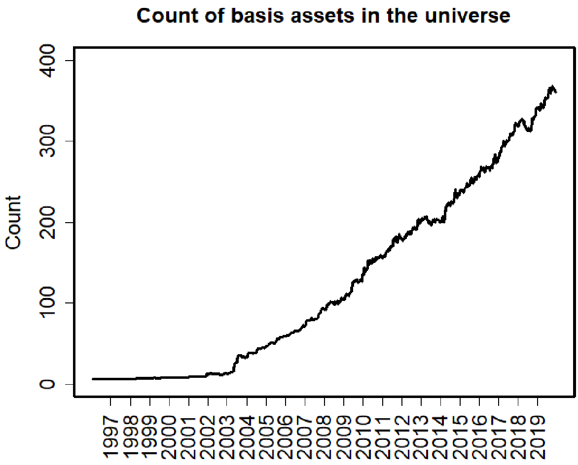 Figure 1: The expansion of the ETF universe providing a rich "basis" for the AMF model.
The Smoking Gun: Different Loadings
The study finds that the anomaly "disappears" when you look through the lens of the AMF model.
- Low-Volatility Portfolios: Load heavily on Bonds, Consumer Staples, and Real Estate. During the study period (2008-2018), these sectors performed exceptionally well in equilibrium.
- High-Volatility Portfolios: Load on Materials, Precious Metals, and Biotech.
When the authors adjusted for these specific ETF-based risks, the "excess return" of the low-volatility portfolio vanished. The anomaly wasn't alpha; it was just the Beta of the sectors it happened to be invested in.
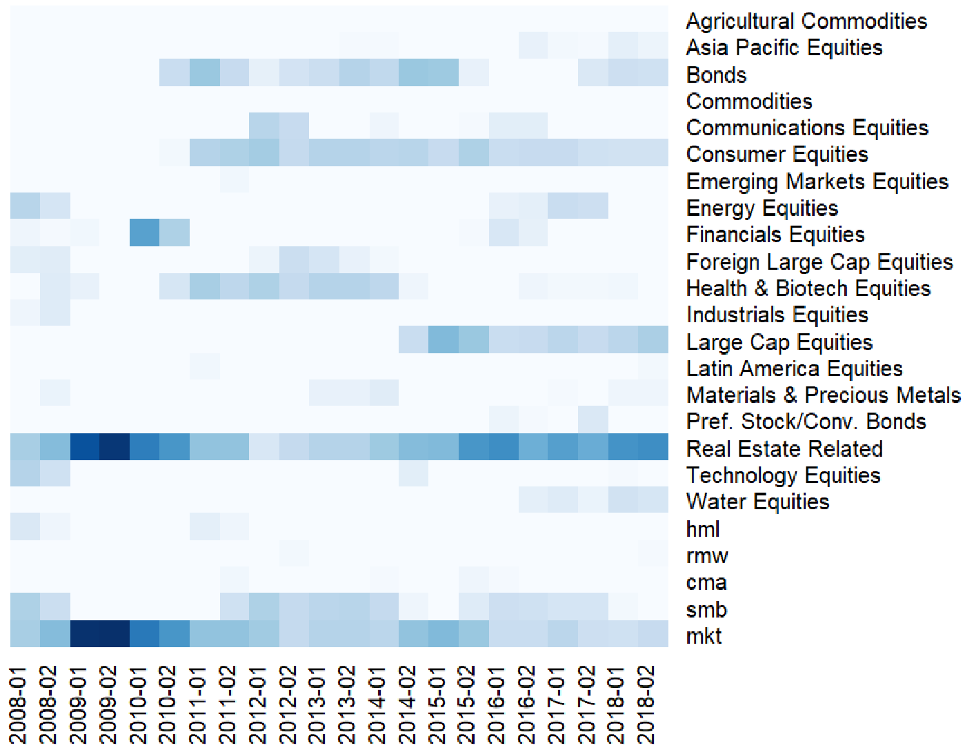 Figure 2: Heatmap showing that Low-Volatility and High-Volatility portfolios live in different "factor neighborhoods."
Experimental Results
The statistical evidence is overwhelming:
- Residual Alpha: In the FF5 model, the p-value for the difference in residuals between low and high vol was nearly zero (anomaly remains). In the AMF model, the p-value was 1.00, meaning the model perfectly explained the difference.
- Predictive Power: AMF achieved an Out-of-Sample of 0.973, outperforming FF5 and proving the model isn't just overfitting noise.
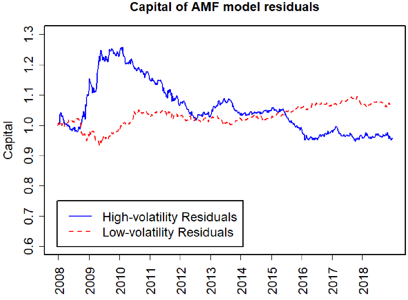 Figure 3: Cumulative residuals under the AMF model show the anomaly virtually disappearing.
Critical Insight & Conclusion
Takeaway: The low-volatility anomaly is a symptom of model misspecification. By moving from static 5-factor models to adaptive, high-dimensional models (AMF), we find that "abnormal" returns are actually just compensation for risks that we previously failed to label.
Limitations: The model relies on a liquid ETF universe. Its effectiveness in markets with fewer "basis assets" (like emerging markets or specific small-caps) remains a secondary area for research. Furthermore, the selection of the 3-year rolling window assumes "local stationarity," which may break during extreme tail events.
In the world of Modern Portfolio Theory, this paper acts as a bridge: validating that markets are more efficient than they look, provided your "microscope" (the AMF model) has enough resolution.