TL;DR

In the world of spatial statistics, the Matérn covariance is king. But a mathematical mystery has persisted for years: in exactly four dimensions, can we tell the difference between a field that is "very bumpy but short-ranged" and one that is "smooth but long-ranged" if we only have one densifying patch of data? This paper finally says yes. By looking at the "faint echoes" in the high-frequency spectrum, the author proves that these models are fundamentally different (mutually singular), completing the dimensional map of Matérn identifiability.

Context: The Identifiability Phase Transition

When we observe a Gaussian Random Field (GRF) on a fixed domain (like a square in $\mathbb{R}^d$) and take more and more samples within that same square—a process called infill asymptotics—we face a limit. For years, we've known a strange truth:

• $d \leq 3$: You cannot distinguish variance ($\sigma^2$) from range ($\alpha$). They are tangled in a single "microergodic" parameter.
• $d > 4$: You can distinguish them perfectly as the sample density goes to infinity.
• $d = 4$: The "Critical Case." The math was too close to call—until now.

The "Why": Why is Dimension 4 so Special?

The difference between two Matérn models with the same microergodic parameter $m = \sigma^2 \alpha^{2 u}$ appears in the high-frequency tail of their spectral densities.

In lower dimensions, the "mismatch" between two models is so small that it's essentially noise—the measures are equivalent. In higher dimensions ($d > 4$), the mismatch is huge. In $d=4$, the mismatch accumulates logarithmically. Like a slow leak in a bucket, it takes a long time to notice, but eventually, the difference becomes infinite.

Methodology: Probing the Spectrum

The author doesn't just look at the raw data. He uses localized Fourier coefficients. By applying a smooth "window" (cutoff function $\chi$) to the field and then taking a Fourier Transform, we can isolate specific frequency bands.

The localized coefficient $X_k$ acts as a "probe" for frequency $k$.

The core of the proof lies in constructing a statistic $T_N$: $$T_N = \frac{1}{L_N} \sum_{k \in \Lambda_N} \delta_k \left(\frac{|X_k|^2}{v_1(k)} - 1\right)$$

This $T_N$ is a "score-type" statistic. Under Model 1, its average is 0. Under Model 2, its average is 1. Because the variance of this statistic shrinks as we look at more frequencies (at a rate of $1/\log N$), the two models eventually drift apart until they no longer overlap.

Experimental Evidence

The author validates this theory with simulations in $d=4$. Even when the parameters $\alpha_1=1$ and $\alpha_2=1.2$ are very close, the empirical distribution of the $T_N$ statistic shows a clear separation as the frequency shell increases.

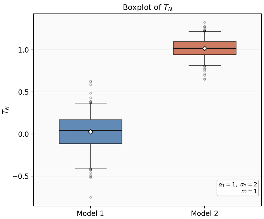Figure 1: Distribution of $T_N$ showing clear separation between Model 1 (centered at 0) and Model 2 (centered at 1).

Deep Insights & Takeaways

The most profound takeaway is the Spectral Probing Framework. While previous attempts (like Anderes' higher-order increments) focused on physical space, this spectral approach provides a much cleaner environment to manage the "off-diagonal" correlations that usually plague spatial data.

Is it useful for AI? Absolutely. As we move toward Physics-Informed Neural Networks (PINNs) and large-scale spatial modeling (like climate AI or medical imaging in 3D/4D), understanding whether our models are over-parameterized is crucial. This paper tells us that in 4D (spacetime!), the range and variance parameters are not just "theoretical constructs"—they are physically distinct and estimable.

Conclusion

By settling the $d=4$ case, this work provides a rigorous mathematical closing to a decades-old question. It reminds us that in the "borderline" cases of mathematics, the signal might be weak (logarithmic), but with the right spectral "microscope," it is undeniable.