Unmasking the Culprit: Rumor Source Identification in Time-Varying Social Networks

TL;DR

Pinpointing where a rumor started is a race against time, exacerbated by the fact that social network connections are constantly shifting—people go offline, move physically, and change social circles. This paper presents the first dedicated framework for source identification in Time-Varying Social Networks. By combining a "Reverse Dissemination" suspect-filtering process with a Maximum Likelihood (ML) estimation based on a microscopic SIR model, the researchers can reduce the search area by up to 90% and identify sources with surgical precision.

Background: The Static Network Fallacy

Most existing "Source Identification" algorithms treat social networks like frozen maps. They rely on static spanning trees or node centrality (like the Jordan Center). However, real-world networks are fluid. If a rumor spreads via Bluetooth at a conference, the "topology" changes every time someone walks to a different room. Traditional models break down here because a path that existed at 10:00 AM might be gone by 10:05 AM.

Methodology: The Detective’s Two-Step

The authors solve this by introducing a two-stage approach inspired by criminology:

1. Reverse Dissemination (Narrowing the Suspects)

Instead of calculating the likelihood for every single node in a million-user network (a scalability nightmare), they perform a "Reverse Dissemination." They treat known infected nodes as starting points and spread "reverse rumors" backward through time-integrated windows.

• The Logic: A true source must be able to reach all currently observed infected nodes. If a node cannot "receive" a reverse rumor from all observed targets, it is acquitted.

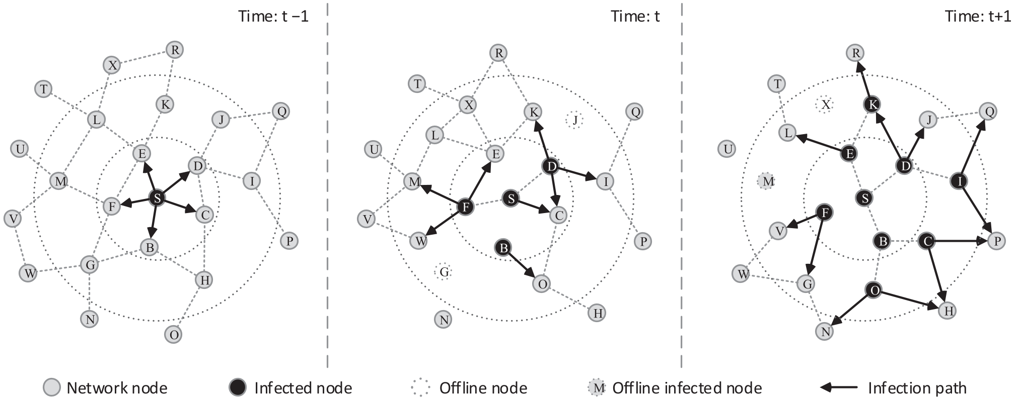Fig 1: Illustrating how time-integrating windows (t1, t2, t3) capture the temporal evolution of contacts.

2. Microscopic ML Estimation (Identifying the Source)

Once a small pool of suspects is identified, the system uses a microscopic SIR (Susceptible-Infected-Recovered) model. It calculates the probability of each suspect producing the exact "observation" (Wavefront, Snapshot, or Sensor data) we see today.

The likelihood $L(u,t)$ is computed as the sum of log-probabilities of all observed nodes being in their specific states (Susceptible, Infected, or Recovered), given a suspect $u$ started the rumor at time $t$.

Handling Different Clinical Observations

The paper brilliantly categorizes three real-world scenarios:

• Wavefront: We only see the "leading edge" of the rumor.
• Snapshot: A frozen moment in time where we see who is currently infected vs. recovered.
• Sensor: A few "monitor" nodes that record the exact time they were hit by the rumor.

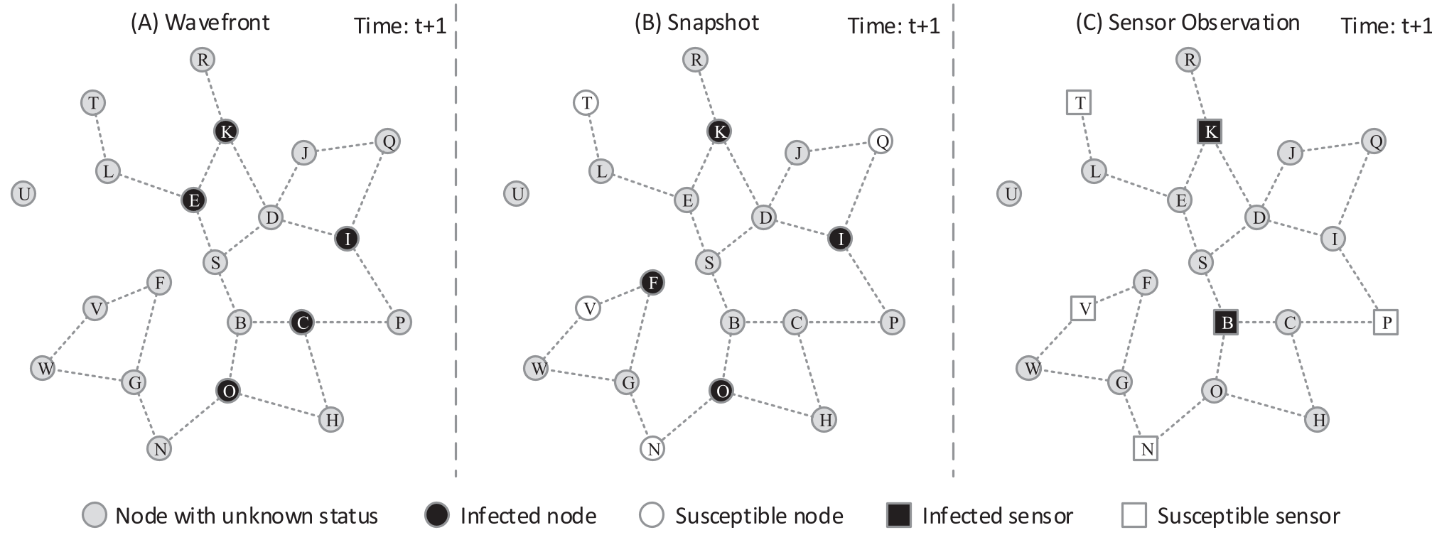Fig 2: Three observation types: (A) Wavefront, (B) Snapshot, (C) Sensor.

Experimental Results & SOTA Comparison

The authors tested their method on four diverse datasets, including MIT Reality (Bluetooth contacts) and Enron Email logs.

• Efficiency: In the MIT dataset, the search area was narrowed to just 5-20% of the total network.
• Accuracy: In Snapshot observations, the accuracy of identifying the exact source hit 70-80% in several datasets.
• Error Distance: Even when the exact node wasn't found, the "estimated source" was usually within a 1-2 hop radius of the truth, which is significantly better than the 3-4 hop error distance of prior tree-based methods.

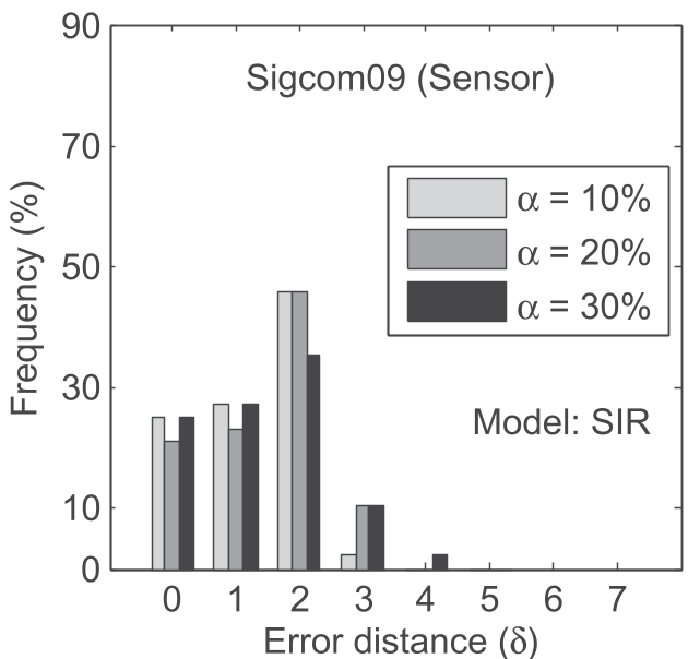Fig 3: Distribution of error distance (d) in the MIT Reality dataset. Note the high frequency at d=0 (exact match).

Critical Insight: Why it Works

The "Secret Sauce" is the Microscopic SIR Model. By analytically deriving the transition probabilities for each node at each discrete time step, the model accounts for the duration and sequence of contacts. In a time-varying network, the order of interactions is as important as the connections themselves. This model captures the "temporal flow" that static centralities miss.

Summary & Future Outlook

This work marks a milestone in digital forensics for social networks. By moving away from static assumptions, it provides a tool actually usable in dynamic environments like mobile ad-hoc networks or fast-moving social media trends.

Limitations noted: The current model uses discrete windows. Moving to continuous-time models could further improve accuracy. Furthermore, as rumors often jump platforms (e.g., from Facebook to Twitter), investigating interconnected network sources is the next logical frontier.

Takeaway: In the fight against misinformation, understanding the when is just as important as the who.