Beyond Snapshots: Scaling Temporal Centrality with EBETS

    ## TL;DR
    In dynamic social networks, being "important" is a transient state. Current methods for measuring this importance (Betweenness Centrality) are slow because they treat time as a series of expensive, redundant static snapshots. This paper introduces **EBETS**, an algorithm that uses **Epoch-points** to forecast exactly when a network's shortest-path structure will change, allowing for order-of-magnitude speedups in temporal analytics.

    ## The Illusion of the Static Network
    Traditional Social Network Analysis (SNA) often collapses time into a single snapshot. However, in reality, social links are "Temporally Detailed" (TD). An email sent at 10:00 AM cannot be part of an information flow that started at 11:00 AM. 

    The challenge is that Betweenness Centrality depends on **Shortest Paths**. In a TD network, the "shortest" path between Person A and Person B might flip from Person C to Person D as time progresses. Calculating this flip at every single minute is a computational nightmare.

    ## The Motivation: Why Dijkstra Fails in Time
    The core issue is **Non-Stationary Ranking**. In a standard graph, Dijkstra's algorithm works because if a path is optimal, its sub-paths are also optimal. In a time-varying network, this ranking shifts. Prior works attempted to solve this by:
    1.  **Re-computing** from scratch (highly redundant).
    2.  **Snapshotting** (loses fine-grained detail).
    3.  **Conservative heuristic updates** (like the LTT algorithm), which still perform more work than necessary.

    ## Methodology: The Power of the Epoch-Point
    The authors propose a "Lazy Strategy" to find **Epoch-points**—the specific moments in time where the shortest path tree rooted at a node actually changes.

    ### The TD Priority Queue
    To find these points on-the-fly, they engineered a **Temporally-Detailed (TD) Priority Queue**. Unlike a standard queue that stores scalar costs, this queue stores **Path-functions** (time-series of costs).
    
    *   **Forecast-Epoch-Point Operation**: This is the "secret sauce." When the algorithm extracts a minimum-cost path, it looks ahead in the time-series to find the earliest intersection point with other candidate paths. This intersection is the next "Epoch-point."

    ![Overall Execution Trace](https://cdn.atominnolab.com/wisdoc/images/20260606-efb1f3fd-02ae-4915-8f9c-9aa7055862ca/page_016_block_009.png)
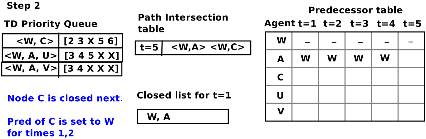
    *Fig 1: The EBETS execution trace showing how path functions are compared to identify valid time intervals for a specific shortest path tree.*

    ## Experiments: Scaling to Real-World Data
    The researchers tested EBETS against the LTT algorithm and a baseline Dijkstra adaptation using three distinct datasets: University Emails, WikiVote, and Foursquare check-ins.

    ### Key Findings:
    *   **Scalability**: EBETS outperformed alternatives by an order of magnitude, especially as the length of the time interval ($\lambda$) increased.
    *   **Wait-Time Robustness**: The algorithm's performance remained stable regardless of the "maximum wait allowed" (the time information can sit at a node).

    ![Performance Comparison](https://cdn.atominnolab.com/wisdoc/images/20260606-efb1f3fd-02ae-4915-8f9c-9aa7055862ca/page_028_block_003.png)
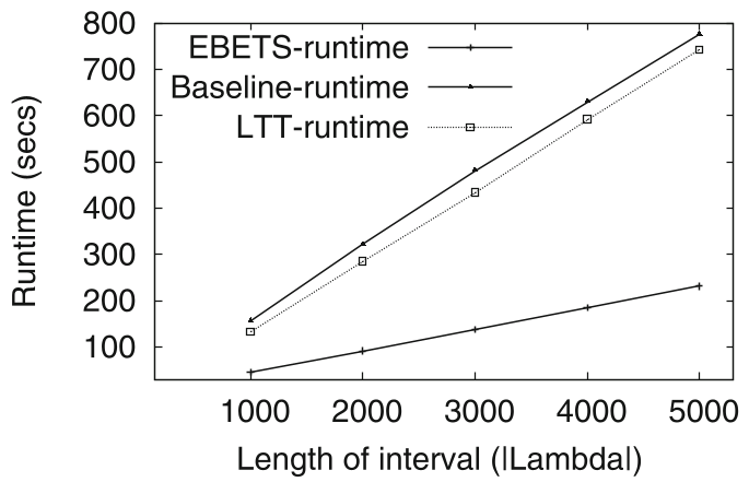
    *Fig 2: Execution time comparison on the University Email dataset. EBETS (lowest line) maintains significantly lower latency compared to LTT and Baseline.*

    ## Comparison: Temporal vs. Traditional Centrality
    The authors performed a fascinating case study. If you just aggregate a day's worth of emails into one snapshot, does the "most central" person match the temporal calculation?
    *   **The Result**: The agreement was only about **60%**. 
    *   **Insight**: Traditional snapshot methods count "impossible paths"—flows of information that violate temporal order. Temporal Betweenness is not just a faster metric; it is a more **accurate** reflection of how influence actually spreads.

    ## Critical Analysis & Conclusion
    **Takeaway**: EBETS effectively bridges the gap between high-fidelity temporal modeling and computational feasibility. By treating "topology changes" as first-class citizens (Epoch-points), it avoids the brute-force repetition of snapshot-based analysis.

    **Limitations**: The algorithm's performance advantage depends on the "Change Probability." If a network is hyper-dynamic (the shortest path tree changes every single second), the number of epoch-points approaches the number of time steps, and the speedup diminishes.

    **Future Outlook**: The epoch-point paradigm could be extended to other metrics like Closeness Centrality or even repurposed for dynamic routing in physical transportation systems, where "traffic" creates similar non-stationary path rankings.