How Multi-Token Prediction Teaches Transformers to Plan: Reverse Reasoning, Gradient Decoupling, and Why NTP Falls Short

Executive Summary

TL;DR

This paper asks a deceptively simple question: why does Multi-Token Prediction (MTP) help reasoning? Empirically, the answer is clear: MTP beats standard Next-Token Prediction (NTP) on graph path-finding, Countdown, and SAT. But the real contribution is deeper: the authors show that MTP changes the optimization geometry of training, not just the supervision density.

Their core theoretical result is that MTP induces a two-stage reverse reasoning circuit. Instead of predicting the next step from the current local prefix, the model first locks onto the end node, then reconstructs the required path backward through intermediate structure. This becomes possible because MTP provides a decoupled gradient signal to early layers, while NTP entangles all learning through deeper, untrained layers.

In short: MTP is not merely a stronger loss; it is an optimization bias toward planning.

Positioning in the Literature

This is best viewed as a mechanistic theory paper with empirical validation, not just another benchmark-improvement paper. Prior work showed MTP helps on reasoning-heavy tasks and is useful in large-scale systems, but this paper explains why a future-token objective can induce a qualitatively different internal algorithm. That makes it more important than a routine SOTA increment: it links objective design to the emergence of interpretable reasoning circuits.

---

Problem & Motivation

Why NTP is a poor fit for planning

Standard autoregressive language modeling uses:

[ \mathcal{L}{\mathrm{NTP}}( heta) = - \frac{1}{T} \sum{t=1}^{T} \log p_{ heta}(x_t \mid x_{1:t-1}). ]

This objective is locally natural, but planning is not a local problem. In planning tasks, the correct current token often depends on future global consistency, not just immediate prefix continuation.

The paper highlights two failures of NTP:

• Local shortcut exploitation: with teacher forcing, the model sees ground-truth previous answer tokens and can often continue them without solving the underlying problem.
• Entangled optimization: gradients reaching early layers must pass through deeper layers, so the signal needed to learn a planning primitive is noisy and poorly aligned.

That combination is toxic for tasks like path-finding, Countdown, and SAT, where the first correct move depends on a valid full solution structure.

The Clever Hans issue is real, but incomplete

In the star-graph task, NTP can cheat. Once the previous node on the path is revealed in the prefix, the model can just follow the outgoing edge. Bachmann & Nagarajan called this the Clever Hans cheat.

But this paper makes an important correction to that story: disabling the shortcut is not the whole explanation.

The binary-tree setup removes much of that trivial dependence because the model must make meaningful decisions repeatedly. Yet MTP still outperforms NTP. So the real issue is not merely shortcut removal. The deeper issue is:

• what kind of reasoning circuit the objective encourages,
• and whether gradient descent can actually discover it.

The authors’ intuition

The paper’s intuition is elegant:

Planning may be easier if the model reasons from the goal backward.

That is exactly what path-finding often looks like algorithmically. If you know the destination, finding the node that points into it is easier than greedily expanding forward with uncertain local evidence.

The surprising claim is that MTP naturally pushes Transformers toward this reverse computation, even though inference still uses ordinary autoregressive generation.

---

Methodology - The Core

From NTP to MTP

MTP with lookahead (k) predicts multiple future tokens from the same prefix:

[ \mathcal{L}{\mathrm{MTP}}^{(k)}( heta) = - \frac{1}{T} \sum{t=1}^{T} \frac{1}{k} \sum_{m=1}^{k} \log p_{ heta,m}(x_{t+m} \mid x_{1:t}). ]

Two details matter here:

• training uses multiple independent heads over a shared backbone,
• inference still emits one token at a time, usually from the first head.

So the benefit is not due to a new decoding algorithm. It comes from a different training signal.

Experimental setup in one sentence

The authors evaluate MTP on:

• star graph path-finding,
• binary tree path-finding,
• Countdown,
• 3-SAT,

and then build a formal analysis on a two-layer disentangled Transformer for a minimal star-graph task.

---

The empirical story: MTP consistently improves planning

The first half of the paper is empirical, and the message is very consistent.

1. Star graph: MTP succeeds where NTP saturates

On the 2-path 5-node star graph:

• NTP stays around 50%
• 2-MTP reaches 100% with 0.5M samples

This is already striking because just one additional future token is enough to qualitatively change learning behavior.

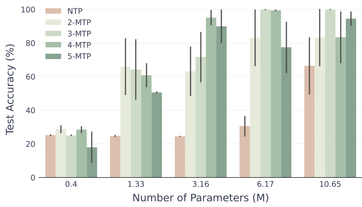
The key takeaway is not merely that MTP is better. It is that NTP appears trapped in a bad solution family, while MTP scales into the correct one.

2. Binary tree: MTP still wins even without easy cheating

The binary tree result is conceptually more important than the star graph.

If MTP only helped because it disabled the teacher-forcing shortcut, then once the shortcut disappears, the gap should vanish. It does not.

Instead:

• NTP begins to improve with more data and parameters,
• but MTP remains stronger, especially in limited-data and limited-capacity regimes.

That suggests MTP is doing more than preventing cheating. It is changing the optimization trajectory toward a more learnable planning algorithm.

3. Countdown and 3-SAT: the effect survives on more realistic combinatorial tasks

Table 1 shows the same pattern on harder tasks:

• Countdown: 60.27 → 64.93 from NTP to 7-MTP
• 3-SAT: 10.40 → 87.47 from NTP to 7-MTP

The SAT jump is especially dramatic. SAT requires a globally consistent assignment; local greedy continuation is fundamentally fragile. So this is exactly the kind of domain where a reverse-planning bias should matter.

---

The central mechanism: reverse reasoning

Now comes the most valuable part of the paper.

The authors analyze a two-layer disentangled Transformer on a small star-graph task and prove that MTP supports a reverse reasoning circuit.

The task structure

The model receives:

• a serialized list of graph edges,
• an end node,
• a start node,

and must generate the path ((u_{ ext{star}}, v, u_{ ext{end}})).

The difficult part is predicting the intermediate node (v). To get it right, the model must determine which edge chain connects start to end.

What reverse reasoning means here

The model learns a two-stage strategy:

1. Layer 1 attends to the end node or its immediate predecessor structure.
2. Layer 2 finds the context edge whose destination matches that end node, thereby recovering the intermediate node.

This is “reverse” because the model is not expanding from the start outward. It is anchoring on the destination and tracing backward.

That mechanism is both:

• algorithmically sensible,
• and more interpretable than a diffuse memorization pattern.

Architecture and attention factorization

The disentangled Transformer splits attention logits into:

• content matching via (W_0^{(\ell)}),
• positional bias via (W_1^{(\ell)}).

This leads to a clean decomposition:

[ A^{[\ell]} := Z W_0^{(\ell)} Z^ op + W_1^{(\ell)}. ]

The simplification matters because it isolates what each layer is learning:

• Layer 1 can specialize into a predecessor pointer
• Layer 2 can specialize into content matching

That separation is exactly what MTP’s gradients encourage.

Theorem-level takeaway

The paper’s Theorem 1 identifies a stationary configuration where:

• Layer 1 points to the predecessor,
• Layer 2 matches the end node to its context occurrence.

Corollary 1 then shows this circuit is constructively realizable by explicit weights. So the issue is not representational capacity. The model class can represent the correct algorithm.

The real question is:

Why does MTP find this circuit while NTP does not?

---

Why MTP finds the circuit: gradient decoupling

This is the core insight of the paper.

The shallow MTP head provides a clean signal

For the lookahead-2 case, MTP includes a shallow loss term (L_2) whose gradient depends only on Layer 1:

[ \mathrm{d} \mathcal{L}_2 ext{ involves only } W_0^{(1)}, W_1^{(1)}, ext{ and is independent of Layer 2.} ]

That is the gradient decoupling property.

This matters because early in training, deeper layers are effectively random. Under NTP, any signal for Layer 1 must backpropagate through untrained Layer 2, so the gradient is misaligned. Under MTP, Layer 1 gets a direct objective and can first learn a useful primitive on its own.

The two-phase learning picture

Theorem 2 formalizes a cascaded optimization process.

Phase I: learn the predecessor pointer

Using the shallow head, Layer 1 learns a universal predecessor-shift pattern:

• attention concentrates on the token at offset (-1),
• i.e. each position points to its immediate predecessor.

In the star-graph setup, this causes the last query to focus on the prompt position containing the end node.

Phase II: solve content matching

Once Layer 1 is stable, Layer 2 only has to perform a contrastive content-matching problem:

• identify where the end node appears in the graph edges,
• suppress the distractor prompt copy of the same end node,
• recover the intermediate predecessor edge.

This decomposition is crucial. MTP turns one hard coupled problem into two easier subproblems.

Why NTP fails: the gradient points the wrong way

Theorem 3 is perhaps the cleanest theoretical punchline.

Under pure NTP near initialization:

• the uninitialized Layer 2 effectively averages over all positions,
• the target intermediate node appears somewhere in the context,
• but not at the predecessor position.

So the NTP gradient tells Layer 1 to spread attention over the context where the target may occur, instead of sharpening it into the predecessor pointer.

In the paper’s words, NTP actively repels the predecessor-pointing solution.

That is a much stronger claim than “NTP is noisy.” It says NTP is structurally biased toward the wrong early learning dynamics on this task.

---

Experiments & Results

A closer reading of the results

Star graph scaling

The most memorable number in the paper is this:

• 2-MTP reaches 100%
• NTP stays at 50%

This is not a marginal gain. It is evidence of two different solution regimes.

Interpretation:

• NTP learns a brittle local heuristic.
• MTP crosses into a qualitatively different planning strategy.

Binary tree scaling

Binary trees are important because they weaken the shortcut explanation.

What we learn:

• NTP can eventually improve when enough data/model scale is available.
• MTP gets there more reliably and sample-efficiently.

Interpretation:

• MTP is not creating a new capability from nowhere.
• It is making the right algorithm easier to find.

Countdown and SAT

These tasks make the paper more than a synthetic-theory exercise.

For Countdown, the first token commits the model to a computation tree.
For SAT, the first assignment propagates constraints globally.

These are exactly the settings where a future-aware objective should help, because the local next token is only meaningful relative to a valid future plan.

Full-scale Transformer validation

The authors also test a standard 8-layer 8-head Transformer on a larger star-graph setup.

Results:

• NTP: 97% train / 20% test
• 3-MTP: 100% train / 100% test

That is a severe generalization gap for NTP and essentially perfect generalization for MTP.

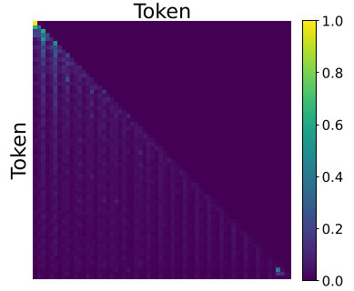
Even more importantly, the attention maps align with the theory:

• NTP attends mainly to the start node
• MTP attends mainly to the end node

This is exactly what reverse reasoning predicts.

Why this evidence is unusually convincing

Many mechanistic papers have one of two weaknesses:

• nice attention visualizations but weak formal theory,
• or elegant theory on toy tasks with little empirical relevance.

This paper is stronger because it offers both:

• a proof that MTP changes gradient flow in a tractable setting,
• and empirical attention behavior in a standard Transformer that mirrors the theory.

That does not mean the theory fully explains modern LLMs, but it does mean the proposed mechanism is more than a toy artifact.

---

Critical Analysis & Conclusion

What the paper really contributes

The real contribution is not “MTP gives better accuracy.” The deeper contribution is:

Training objectives can induce different internal algorithms by reshaping gradient flow.

That is a powerful idea for reasoning research. It suggests capability differences may emerge not only from scale, architecture, or data, but from objective-induced optimization biases.

Why the reverse reasoning story is compelling

The reverse reasoning circuit is compelling for three reasons:

• It is algorithmically natural for planning.
• It is mechanistically visible in attention patterns.
• It is optimization-derived, not manually hard-coded.

This last point matters most. The model is not forced to plan backward at inference. It learns to do so because MTP makes that route easier for gradient descent to discover.

Limitations

The paper is strong, but its boundaries are clear.

• The theory is built on a two-layer disentangled Transformer.
• The main proof focuses on a small star-graph task.
• The key formal result is for lookahead (k=2).
• The analysis does not yet cover:
  • deeper general architectures in full generality,
  • arbitrary graph topologies,
  • finite-time convergence,
  • sequential MTP variants such as those used in some industrial systems.

So one should not overclaim that all MTP gains in frontier LLMs are fully explained by this mechanism.

Open questions

Several natural extensions follow from this work:

• Does reverse reasoning emerge in math and code benchmarks with the same clarity?
• For larger (k), do we get deeper cascades of subproblem decomposition?
• Can objective design produce circuits beyond backward planning, such as search or verification?
• How much of MTP’s benefit in real LLMs comes from optimization, and how much from representation sharing or data efficiency?

Final takeaway

This paper makes a strong case that MTP is an optimization prior for planning. NTP asks the model to continue; MTP asks it to anticipate. That small-looking change alters the gradients enough to make a backward, goal-conditioned reasoning circuit discoverable.

If that thesis continues to hold beyond toy settings, then the implication is substantial:

• better reasoning may require not just bigger models,
• but better training objectives that expose future structure early enough for optimization to latch onto it.

That is a meaningful lesson for both theory and practice.