FriendTNS: Re-evaluating Link Prediction through Transitive Proximity

TL;DR

Recommending "People You May Know" is a staple of modern social media, yet most platforms still rely on shallow metrics like "number of common friends." This paper introduces FriendTNS, an algorithm that captures the "strength" of connections by viewing friendship as a transitive property. By punishing high-degree bridges (which are less likely to signify personal acquaintance) and calculating similarity along the shortest paths, FriendTNS achieves SOTA accuracy while remaining fast enough for real-time applications.

Background & Positioning

In the landscape of graph mining, link prediction is often split into two camps: Local Heuristics (fast but short-sighted like FOAF) and Global Heuristics (accurate but slow like SimRank or RWR). FriendTNS positions itself as a hybrid "middle-ground" solution. It leverages the "Small World" property of social networks to provide deep structural insights without the $O(N^3)$ or $O(N^2)$ overhead of global matrix inversions.

Problem & Motivation: The "Hub" Fallacy

The authors identify a critical flaw in traditional count-based recommendations. If User A is connected to User B through a "hub" (a celebrity or a community page with thousands of followers), that connection is statistically weaker than a connection through a "private" user with only five friends.

Current systems like Facebook often rank all candidates with one common friend equally. FriendTNS argues that:

1. Similarity is inverse to degree: If you share a friend who has 1,000 other friends, that "bridge" is diluted.
2. Transitivity decays: A friend of a friend is a strong candidate; a friend of a friend of a friend is weaker, but still more relevant than a stranger.

Methodology: The Transitive Engine

The core of the paper is the Extended Similarity (esim).

1. Basic Similarity (The Local Build)

Based on the Tanimoto coefficient, the similarity between two neighbors $v_i$ and $v_j$ is defined by the inverse of their degree sums: $sim(v_i,v_j)=\frac{1}{deg(v_i)+deg(v_j)-1}$ This ensures that "hubs" naturally receive lower similarity scores.

2. Transitive Extension (The Global Reach)

For nodes not directly connected, the algorithm finds the shortest path and multiplies the basic similarities along that path: $esim(v_i,v_j)={\prod }_{h=1}^{k}sim(v_{p_h},v_{p_{h+1}})$

3. The FriendTNS Algorithm

The authors utilize a modified Dijkstra approach. To ensure scalability, they introduce a Precision Threshold ($p$). If the product of similarities along a path drops below $p$, the algorithm stops searching that branch. This keeps the computation focused on the target user's local "neighborhood" while still allowing for deep, multihop discovery.

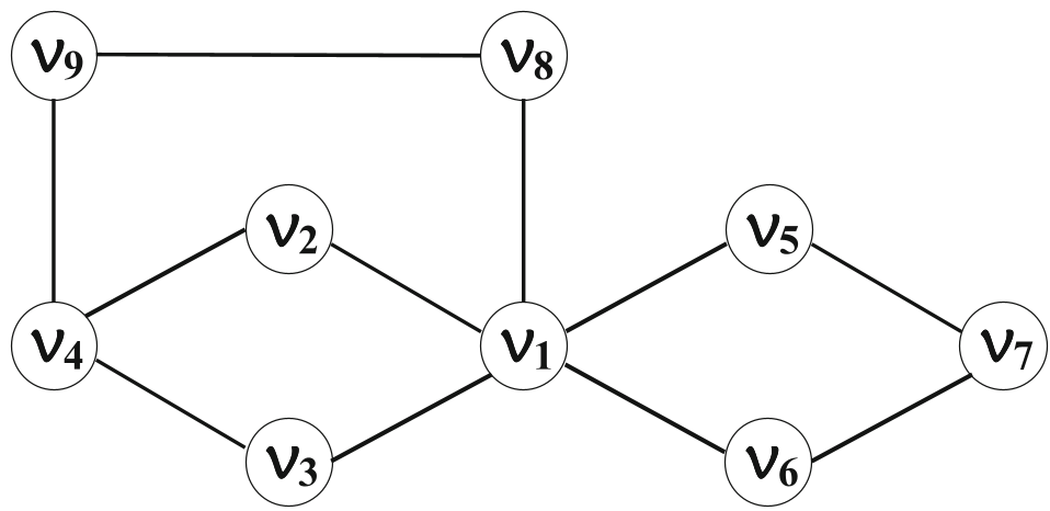Note: The algorithm effectively balances the exploration of the network by pruning weak transitive paths.

Experiments & Results

The authors tested FriendTNS on Facebook (3.7K nodes), Hi5 (63K nodes), and Epinions (49K nodes).

SOTA Accuracy

FriendTNS consistently outperformed Adamic/Adar and RWR. On the Facebook dataset, the precision-recall curve showed a dominant lead, specifically because the high clustering coefficient of Facebook rewards the algorithm's ability to weight local paths intelligently.

Efficiency at Scale

One of the most impressive results is the time complexity. In a synthetic network of 100,000 nodes, FriendTNS was ~10x faster than the standard Shortest Path algorithm and ~14x faster than RWR.

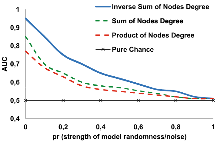Experimental results showing precision vs. different basic metrics.

The Power of "Negative" Info

The paper also explores Signed Networks. By using Status Theory (interpreting directed signs as status differentials) and Balance Theory ("the enemy of my enemy is my friend"), the authors showed that including negative links improved the prediction of positive links (FriendTNS- vs FriendTNS+).

Critical Insight & Conclusion

Takeaway

FriendTNS proves that you don't need expensive matrix operations to capture global graph structure. By treating the graph as a series of decaying transitive similarities, we can achieve high-fidelity recommendations with $O(m+n\log n)$ complexity.

Limitations

• Dynamic Update: While the authors claim incremental updates are possible, frequent edge deletions in high-density graphs may still require significant re-calculations.
• Precision Sensitivity: The choice of $p$ is empirical. In extremely dense graphs, a poorly chosen $p$ might still lead to excessive computation.

Future Outlook

The next logical step is integrating these transitive scores into Graph Neural Networks (GNNs) as an inductive bias, potentially combining the structural precision of FriendTNS with the feature-learning power of deep learning.